We calculated the net worth and return rate of users on Uniswap from the perspective of user addresses. This time, our goal remains the same, but we will include the cash holdings of these addresses in the calculation to obtain the total net worth and return rate.

Author: Zelos

Introduction

In the previous issue, we calculated the net worth and return rate of users on Uniswap from the perspective of user addresses. This time, our goal remains the same, but we will include the cash holdings of these addresses in the calculation to obtain a total net worth and return rate.

The statistical objects this time include two pools, which are:

• usdc-weth (fee: 0.05) on Polygon, pool address: 0x45dda9cb7c25131df268515131f647d726f50608[1], which was also used in the previous analysis
• usdc-eth (fee: 0.05) on Ethereum, pool address: 0x88e6A0c2dDD26FEEb64F039a2c41296FcB3f5640[2], which presents some challenges in data processing due to the inclusion of a native token in this pool

The resulting data is on an hourly basis. Note: Each row of data represents the value at the end of that hour.

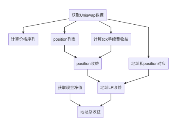
Overall Process

1. Obtain Uniswap data
2. Obtain user cash data
3. Calculate price sequences, i.e., the price of eth
4. Obtain the amount of fees collected on each tick per minute
5. Obtain the list of all positions within the statistical period
6. Establish the relationship between addresses and positions
7. Calculate the return rate for each position
8. Calculate the return rate for each user address as an LP based on the relationship between positions and addresses
9. Combine user cash and LP, and calculate the overall return rate

1. Obtain Uniswap Data

Previously, in order to provide data sources for Demeter, we developed the demeter-fetch tool. This tool can retrieve Uniswap pool logs from different channels and parse them into different formats. Supported data sources include:

• Ethereum RPC: the standard RPC interface of the eth client. Retrieving data is relatively inefficient and requires opening multiple threads.
• Google BigQuery: downloading data from the BigQuery dataset. Although it is updated daily, it is convenient to use and cost-effective.
• Trueblocks chifra: the Chifra service can scrape on-chain transactions and reorganize them, making it easy to export transaction and balance information. However, this requires setting up nodes and services.

The output formats include:

• minute: resampling the transaction information of uniswap swaps into data for each minute, used for backtesting
• tick: recording each transaction in the pool, including swaps and liquidity operations

This time, we mainly obtained tick data to analyze position information, including the amount of funds, per-minute earnings, lifespan, and holders.

These data are obtained from the event logs of the pool, such as mint, burn, collect, and swap. However, the pool's log does not contain token IDs, which makes it impossible for us to locate which position the pool's operation is targeting.

In fact, the equity of Uniswap LP is managed through NFTs, and the managers of these NFT tokens are proxy contracts. The token IDs only exist in the event logs of the proxy. Therefore, to obtain complete LP position information, we need to obtain the event logs of the proxy and then combine them with the event logs of the pool.

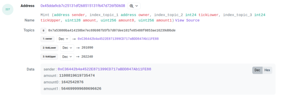
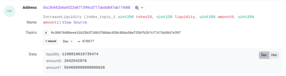
Taking this transaction[3] as an example, we need to pay attention to two logs with log indexes 227 and 229. They are the mint thrown out by the pool contract and the IncreaseLiquidity thrown out by the proxy contract. The amount (i.e., liquidity), amount0, and amount1 between them are the same. This can serve as the basis for association. By associating these two logs, we can obtain the tick range, liquidity, token ID, and the amounts of the two tokens corresponding to this LP behavior.

For advanced users, especially some funds, they may choose to bypass the proxy and directly operate the pool contract. In this case, the position will not have a token ID. In this case, we will create an ID for this LP position in the format of address-LowerTick-UpperTick.

For burn and collect, we can also use this method to find the corresponding position ID for the pool's event. However, there is a problem here. Sometimes the amounts of the two events are not exactly the same, and there may be a slight deviation. For example, in this transaction:

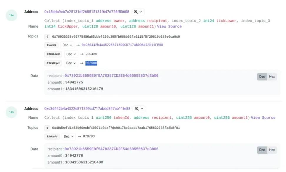
The amount0 and amount1 will have a small difference, although this situation is rare, it is also common. Therefore, when matching burn and collect, we have left some margin for error in the values.

The next issue to address is who initiated this transaction. For withdrawal, we will use the receipt in the collect event as the holder of the position. For mint, we can only obtain the sender from the pool mint event (see the graph with the mint event).

If the user is operating the pool contract, the sender will be the LP provider. However, if it is a regular user operating the contract through the proxy, the sender will be the address of the proxy. This is because the funds are indeed transferred from the proxy to the pool. Fortunately, the proxy will generate an NFT token, and this NFT token will definitely be transferred to the LP provider. Therefore, by monitoring the transfer of the proxy contract (i.e., the NFT token contract), we can find the LP provider corresponding to this mint.

Additionally, if the NFT is transferred, it will cause a change in the holder of the position. We have conducted statistics on this, although this situation is rare. To simplify, we did not consider the transfer of NFTs after minting.

2. Obtain the Cash Holdings of Addresses

The goal of this stage is to obtain the quantity of tokens held by an address at each moment during the statistical period. To achieve this goal, we need to obtain two types of data:

1. The balance of the address at the starting moment
2. The transfer records of the address during the statistical period

By using the transfer records to adjust the balance, we can infer the balance at each moment.

For the balance at the starting moment, it can be queried through the RPC interface. When using an archive node, the balance at any time can be obtained by setting the height in the query parameters. This method can be used to obtain the balance of both native tokens and ERC20 tokens.

Obtaining the transfer records of ERC20 tokens is relatively easy and can be obtained through any channel (BigQuery, RPC, Chifra).

However, obtaining the transfer records of ETH requires retrieval through transactions and traces. Retrieving transactions is relatively straightforward, but querying and processing traces involves a large amount of computation. Fortunately, Chifra provides the function to export ETH balances, which can output a record when the balance changes. Although it can only record the quantity change and not the recipient of the transfer, it still meets the requirements and is the most cost-effective method.

3. Price Retrieval

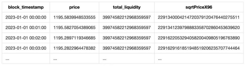
Uniswap is an exchange, and if a token exchange occurs, a swap event is generated. We can obtain the price of the token from the sqrtPriceX96 field and the total liquidity at that time from the liquidity field.

Since our pools all have a stablecoin, obtaining the price in terms of the stablecoin is very easy. However, this price is not absolutely accurate. Firstly, it is influenced by the frequency of transactions. If there are no swap transactions, this price will lag behind. Additionally, when the stablecoin deviates from its peg, there will be a discrepancy between this price and the price in terms of the stablecoin. But in general, this price is accurate enough and is suitable for market research.

Finally, by resampling the token prices, we can obtain a list of prices for each minute.

Additionally, since the liquidity field of the event also includes the total liquidity of the pool at the current moment, we will also include the total liquidity. This will ultimately form a table like the following:

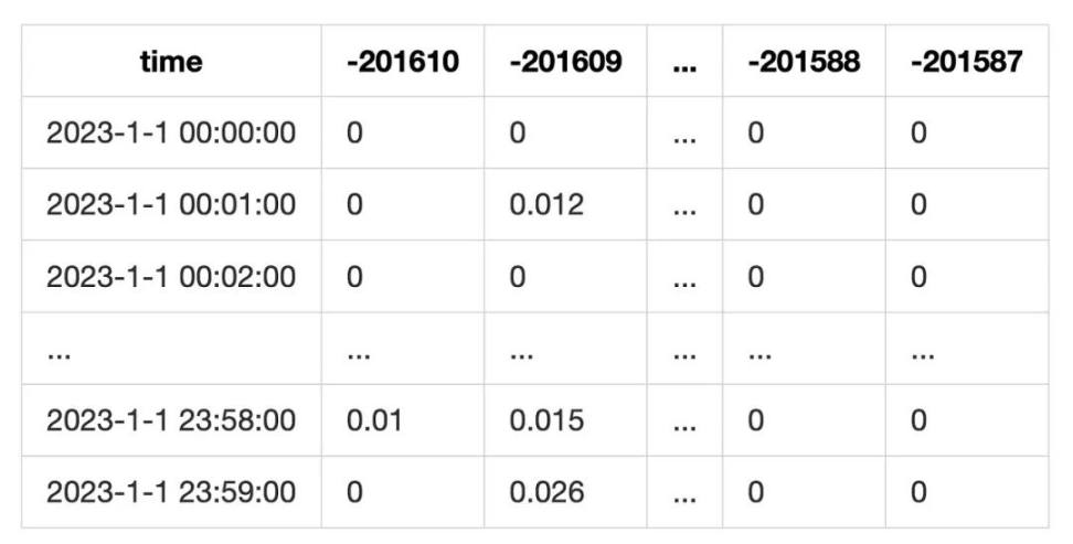
4. Fee Statistics

Fees are the main source of income for positions. Every time a user performs a swap operation on the pool, the corresponding position can receive a certain amount of fees (for the position that includes the current tick). The amount of income is related to the proportion of liquidity, the pool's fee rate, and the tick range.

To calculate the user's fee income, we can record the amount of swap transactions that occurred on each tick of the pool every minute. Then we can calculate the fee income on that tick for the current minute:

This will ultimately form a table like this:

This method of calculation does not consider the situation where the liquidity of the current tick is exhausted during a swap. However, since our goal is to analyze LP using tick ranges, this error can be mitigated to a certain extent.

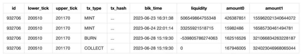
5. Obtain the List of Positions

To obtain the list of positions, we first need to specify the identifier of the position.

• For LPs invested through the proxy, each position will have an NFT, i.e., a token ID, which can serve as the position's ID.
• For LPs directly operating the pool investment, we will create an ID for them in the format address_LowerTick_UpperTick. This way, all positions will have their own identifiers.

Using these identifiers, we can consolidate all the operations of the LPs and form a list describing the entire lifecycle of the positions, such as:

However, it is important to note that the objects of this statistical analysis are from the year 2023, not from the inception of the pools. Inevitably, for some positions, we cannot obtain their operations before January 1, 2023. This requires us to speculate on how much liquidity these positions had at the start of the statistical period. We have adopted an economical method to speculate:

1. Add the liquidity of mint and burn to obtain a number L.
2. If L > 0, i.e., mint > burn, it is assumed that there was some liquidity before the start of the statistical period, and a mint operation will be compensated at the start of the statistical period (January 1, 2023, 0:0:0).
3. If L < 0, it is assumed that there was still liquidity held at the end of the statistical period.

This approach can avoid downloading data before 2023, thus saving costs. However, it will face the issue of submerged liquidity, meaning that if an LP did not make any transactions during the year, it will not be found. However, this issue is not severe. Since the statistical period is one year, we assume that users generally adjust their LP during this period. Over the span of a year, the price of ETH can undergo significant changes, and users have many reasons to adjust their LP, such as when the price exceeds the tick range or when they allocate funds to other DeFi projects. Therefore, as an active user, they will definitely adjust their LP based on the price. For those who keep their funds stagnant in the pool without making adjustments, we consider them to be inactive and not within the scope of the statistics.

Another more complicated situation is when a position minted some liquidity before 2023, then performed some mint/burn operations during the period, and did not burn all the liquidity by the end of the statistical period. Therefore, we can only calculate a portion of the liquidity. In this case, submerged liquidity will affect the estimation of position's fee income, resulting in abnormal yield. The specific reasons will be discussed later.

In the final statistics, there are a total of 73,278 positions on Polygon and 21,210 positions on Ethereum, with abnormal yields not exceeding 10 for each chain, proving that this assumption is reliable.

6. Obtain the Correspondence between Addresses and Positions

Since the ultimate goal of our statistics is the income of addresses, we also need to obtain the correspondence between addresses and positions. Through this association, we can understand the specific investment behavior of users.

In step 1, we did some work to find the associated users for fund operations (mint/collect). Therefore, as long as we find the sender of the mint and the recipient of the collect, we can find the correspondence between positions and addresses.

7. Calculate the Net Value and Yield of Positions

In this step, we need to calculate the net value of each position and then calculate the yield based on the net value.

Net Value

The net value of a position consists of two parts: the LP's liquidity, which is equivalent to the principal of market making. After a user invests funds in a position, the quantity of liquidity does not change, but the net value fluctuates with changes in price. The other part is the fee income, which is independent of liquidity and is stored separately in the fee0 and fee1 fields. The fee net value increases over time.

Therefore, at any minute, combining liquidity with the price of that minute will yield the net value of the principal portion. Calculating the fee income requires using the fee table calculated in the fourth step.

First, use the position's liquidity, divided by the total liquidity of the current pool, as the profit-sharing ratio. Then, add up the fees for all ticks included in the position's tick range to obtain the fee income for that minute.

It can be represented by the formula:

Finally, adding the fee net value to the liquidity net value yields the total net value.

When calculating the net value, we divide the lifecycle of the position based on mint/burn/collect transactions.

1. When a mint transaction occurs, the liquidity increases.
2. When a burn transaction occurs, the liquidity decreases, and the value of the liquidity is converted to the fee field (the pool contract's code also operates in this way).
3. When a collect transaction occurs, it triggers the calculation. The calculation range is from the last collect to the current time, and we calculate the net value and fee income for each minute, resulting in a list.

Finally, we aggregate the net value lists obtained from each collect. Then, we perform resampling and other statistics to obtain the final results.

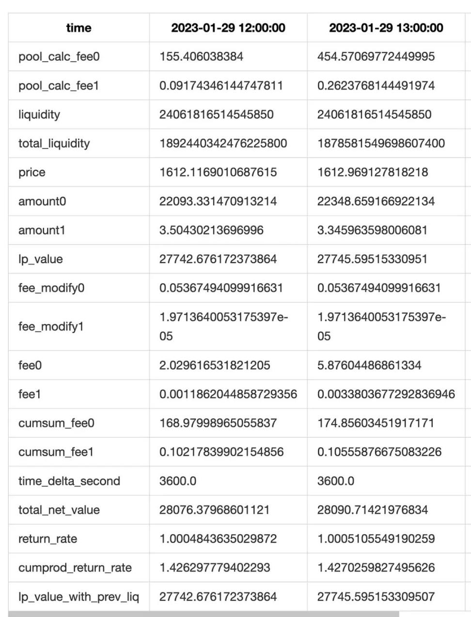
Additionally, to improve accuracy, we have made two optimizations.

First, for hours with transactions (mint/burn/collect), we perform minute-level statistics, while for hours without transactions, we perform hour-level statistics. Finally, we resample the results into hour-level data.

Second, in the collect event, we can obtain the total of liquidity + fees. Therefore, we can compare the actual collected value with our theoretical calculated value to obtain the difference between theoretical and actual fees (in fact, this difference also includes the difference in LP principal, but the error in LP principal difference is very small and can be considered as 0). We will compensate for the fee difference in each row to improve the accuracy of fee estimation (i.e., the feemodify0 and feemodify1 fields in the table above).

Note:

1. When backfilling, we need to weight the distribution of fees based on the current hour's liquidity to avoid situations where the fees for that hour are disproportionately high.
2. Since the data being analyzed is for the entire year of 2023 and not complete data, the phenomenon of submerged liquidity mentioned in section five exists. This will result in actual fees being much higher than theoretical fees, leading to abnormally high yields.

Since each row represents the data at the end of that hour, for positions that have been completely closed, the net value will be 0. In this case, the net value at the time of position closure will be lost. To retain this net value, a line of data with a timestamp of 2038-1-1 00:00:00 has been created at the end of the file, storing the net value at the time of position closure and other data for the needs of other projects' statistics.

Yield

Usually, the yield is calculated by dividing the initial net value by the final net value. However, this method is not applicable here for the following reasons:

1. The yield here needs to be refined to each minute.
2. Since positions may have funds transferred in and out midway, simply dividing the initial and final net values cannot reflect the yield situation.

For problem 1, we can obtain the yield for each minute by dividing the net values for each minute, and then multiplying the yield for each minute cumulatively to obtain the total yield.

However, this algorithm has a serious issue. If there is a calculation error in the yield for any minute, it will lead to a significant deviation in the total yield. This turns the statistical process into a tightrope walk, where there is no room for error. However, the good thing is that this makes any statistical errors very apparent.

For problem 2, if there are fund transfers in and out within a minute, simply dividing the yield directly will still result in unreasonable yields. Therefore, it is necessary to refine the algorithm for calculating the yield for each minute.

Our first attempt was to break down the changes in net value in detail and exclude the changes in funds. We divided the change in net value into several parts: 1) the change in principal due to price, 2) the cumulative fees for that minute, and 3) the inflow and outflow of funds. Obviously, the third part needs to be excluded from the statistics. For this, we formulated the following calculation method:

1. Designate the current minute as "n" and the previous minute as "n-1."
2. Assume that all transfer operations in the current minute occur at the start of the minute (n:0.000 seconds). Therefore, for the remaining time, the net value of the LP remains unchanged, meaning that the net value at n:0.001 seconds is equal to the net value at n:59.999 seconds.
3. The accumulation of fees occurs at the end of this minute, i.e., at n:59.999 seconds.
4. The price and fees at the end of the previous minute (n-1:59.999) are considered as the starting values for the current minute (n:0.000).

Based on these assumptions, the yield for each minute is calculated using the end liquidity / price / fees divided by the start liquidity / price / fees. It can be represented by the following formula, where "f" refers to the algorithm for converting liquidity to net value.

This approach seems promising. It perfectly avoids the variability of liquidity and reflects the impact of price and fees on net value, which is exactly what we expected. However, in practice, it may result in very high yields for certain rows. Upon investigation, we found that the issue arises when withdrawing liquidity. Recall our rule: each row represents the end of the minute/hour. This provides a uniform scale for data statistics, but it is important to note that the meaning of each column is different:

• For the net value column, it represents instantaneous values, i.e., the value at the end of the current minute/hour.
• For the fee column, it represents cumulative values, i.e., the fees accumulated during the current minute/hour.

Therefore, for the hour when liquidity is burned:

• When the LP is burned and the tokens are transferred out, the net value at the end of that hour will be 0.
• However, for the fees, since they are cumulative, at the end of that hour, the fees will be greater than 0.

This causes the above formula to degenerate into:

This situation not only occurs at the end of the position's lifecycle but also when burning a portion of the liquidity, causing changes in the ratio of fee income to the LP's net value.

For simplicity, when there is a change in the net value of the LP, we set the yield to 1. This introduces some error in the calculation of the yield. However, for a position with normal continuous investment, the hours with transactions are relatively few compared to the entire lifecycle, so the impact is not significant.

8. Calculate the Total LP Income for Addresses

With the yield for each position and the correspondence between positions and addresses, we can calculate the yield for each position for user addresses.

The algorithm here is relatively simple. Concatenate the positions for the address at different times. If there is no investment in between, set the net value to 0 and the yield to 1 (because there is no change in net value, so the yield is 1).

If there are multiple positions for the same period, then in the overlapping parts, add the net values to obtain the total net value. When merging the yields, we will weight the merge based on the net value of each position.

9. Merge the Total Income from Cash and LP

Finally, by combining the cash and LP investments held by user addresses, we can obtain the final results.

Merging the net value is simpler compared to the previous step (merging positions). We only need to find the time range for the LP net value, then find the corresponding cash holdings for that time range, and then find the ETH price to obtain the total net value.

For the yield, we use the algorithm of calculating the yield for each minute and then multiplying them cumulatively. Initially, we used the erroneous yield calculation algorithm mentioned in section seven. This required separating the fixed part for each minute (including the cash quantity in cash and the liquidity in LP) from the variable part (price changes, cumulative fees, fund transfers). Relative to the statistics for positions, this method is much more complex because for fund inflows and outflows in Uniswap LP, we only need to pay attention to mint and collect events. However, retracing cash holdings is very complicated. We need to distinguish whether the funds are transferred to the LP or to an external source. If they are transferred to the LP, the principal portion can remain unchanged, but if they are transferred externally, the quantity of the principal needs to be adjusted. This requires tracking the target addresses for ERC20 and ETH transfers, which is very cumbersome. Firstly, during mint/collect events, the transfer address may be the pool or the proxy. What's even more complex is the transfer of ETH. Since ETH is a native token, some transfer records can only be traced through trace records. However, the volume of trace data is too large and exceeds our processing capacity.

The final straw that broke the camel's back was when we discovered that the net value for each row represents the instantaneous value for that hour, while the fees represent the cumulative value for that hour. Physically, they cannot be directly added together. This issue was only discovered very late.

Therefore, we abandoned this algorithm and instead adopted the method of dividing the net value at the end of one minute by the net value at the end of the previous minute. This method is much simpler. However, it also has a problem: when there are fund transfers, the yield can still be unreasonable. From the discussion above, we learned that it is very difficult to trace the direction of fund transfers. Therefore, here we sacrifice some accuracy and set the yield to 1 when there are fund transfers.

The remaining issue is how to identify fund inflows and outflows within the current hour. Initially, the algorithm we thought of was very simple: use the token balance from the previous hour and the current price to calculate what the net value would be for that hour if holding those tokens. Then, subtract the calculated value from the actual value. When the difference is not equal to zero, it indicates fund inflows or outflows. It can be represented by the formula:

However, this algorithm overlooks the complexity of Uniswap LP. In LP, the quantity of tokens changes with price fluctuations, and the net value also changes accordingly. Additionally, this method does not consider changes in fees. As a result, the estimated value and the actual value have an error of around 0.1%.

To improve accuracy, we further refined the composition of funds, separately calculating the change in LP value and considering the fees.

Through this method, the error in the estimated value can be controlled to within 0.001%.

Additionally, we have limited the decimal points of the data to avoid extremely small numbers (usually below 10^-10) being divided. These small numbers are errors accumulated from various calculations and resampling. If not handled properly, direct division can lead to error amplification, resulting in significant distortion of the yield.

Other Issues

Native Token

In this round of statistics, the USDC-ETH pool on Ethereum was included, where ETH is the native token and requires some special handling.

ETH cannot be used in DeFi and must be converted to WETH. Therefore, this pool is actually a USDC-WETH pool. For users directly interacting with the pool, they can deposit and withdraw WETH from this pool, similar to regular pools.

However, for users adding LP through a proxy, they need to include ETH in the transaction value and transfer it to the proxy contract. The contract will then convert these ETH to WETH and deposit them into the pool. When collecting, USDC can be directly transferred to the user, but ETH cannot be directly transferred and needs to be withdrawn from the pool to the proxy, then converted to ETH by the proxy contract, and finally sent to the user through an internal transfer. An example of this transaction can be seen here [4].

Therefore, the USDC-ETH pool differs from regular pools only in the inflow and outflow of funds. This only affects the matching of positions and addresses. To address this issue, we retrieved all NFT transfer data from the creation of the pool and then found the holders of the corresponding positions through the token ID.

Missing Positions

In the statistics, some positions did not make it into the final list. These positions have certain special characteristics.

A large portion of these are MEV (Miner Extractable Value) trades, which are purely arbitrage trades and not made by regular investors, so they are not within the scope of our statistics. Additionally, it is also difficult to track them in actual statistics, as it requires trace-level data. Here, we used a simple strategy to filter out MEV trades, which is if the time from start to finish is less than one minute. In fact, since our data has a maximum precision of one minute, if a position exists for less than one minute, it cannot be included in the statistics.

Another possibility is that the position did not have a collect transaction. As seen in step 7, our yield calculation is triggered by the collect operation. Without a collect operation, the previous net value and yield will not be calculated. Under normal circumstances, users would choose to harvest the LP yield or principal in a timely manner. However, there may be some special users who want to keep their assets in the Uniswap pool for fee0 and fee1. For these users, we also consider them as special users and do not include them in the statistics.

References

[1] 0x45dda9cb7c25131df268515131f647d726f50608: https://polygonscan.com/address/0x45dda9cb7c25131df268515131f647d726f50608

[2] 0x88e6A0c2dDD26FEEb64F039a2c41296FcB3f5640: https://etherscan.io/address/0x88e6A0c2dDD26FEEb64F039a2c41296FcB3f5640

[3] This transaction: https://polygonscan.com/tx/0x0194473ed30555c244bc55f5b2ca70097ccd9cfbb819c92c7d14fcf46839397f#eventlog

[4] This transaction: https://etherscan.io/tx/0x6178aeef0406f184385f5600b1d49a387a7a987ce461274addbe75ae95a4f40d#eventlog

免责声明：本文章仅代表作者个人观点，不代表本平台的立场和观点。本文章仅供信息分享，不构成对任何人的任何投资建议。用户与作者之间的任何争议，与本平台无关。如网页中刊载的文章或图片涉及侵权，请提供相关的权利证明和身份证明发送邮件到support@aicoin.com，本平台相关工作人员将会进行核查。