Title: Vitalik Buterin

Translation: Kate, MarsBit

This article is mainly aimed at readers who are roughly familiar with the cryptography of 2019, especially SNARK and STARK. If you are not, I suggest you read these articles first. Special thanks to Justin Drake, Jim Posen, Benjamin Diamond, and Radi Cojbasic for their feedback and comments.

Over the past two years, STARK has become a critical and irreplaceable technology that can effectively provide easily verifiable cryptographic proofs for very complex statements (e.g., proving the validity of Ethereum blocks). One key reason is the small field size: SNARK based on elliptic curves requires you to work with 256-bit integers to be secure enough, while STARK allows you to use smaller field sizes, making it more efficient: first is the Goldilocks field (64-bit integers), then Mersenne31 and BabyBear (both 31 bits). Due to these efficiency improvements, using Goldilocks, Plonky2 is several hundred times faster in proving various computations than its predecessors.

A natural question is: can we lead this trend to a logical conclusion by directly building a faster proof system by operating on zero and one? This is exactly what Binius is trying to do, using many mathematical tricks that make it fundamentally different from SNARK and STARK three years ago. This article explains why small fields make proof generation more efficient, why binary fields have unique powerful capabilities, and the techniques Binius uses to make proofs on binary fields so effective.

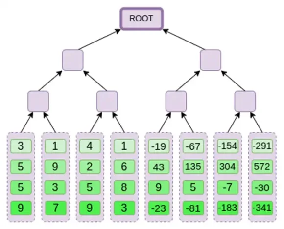
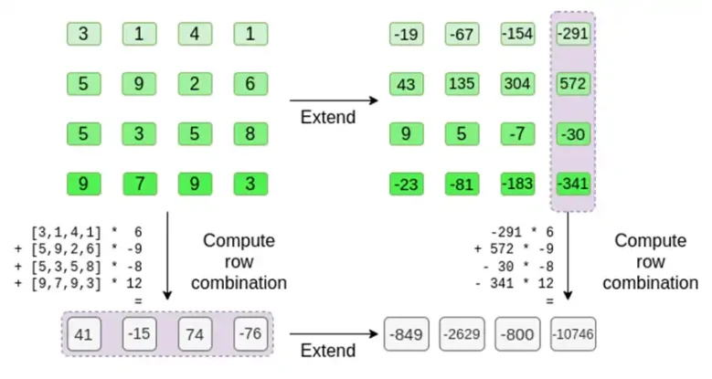
Binius, at the end of this article, you should be able to understand each part of this diagram.

Review: Finite Fields

One of the key tasks of cryptographic proof systems is to operate on a large amount of data while keeping the numbers small. If you can compress a statement about a large program into a mathematical equation containing only a few numbers, but those numbers are as large as the original program, then you have gained nothing.

To perform complex arithmetic while keeping the numbers small, cryptographers often use modular arithmetic. We choose a prime number "modulus" p. The % operator means "take the remainder": 15%7=1, 53%10=3, and so on. (Please note that the answer is always non-negative, so for example, -1%10=9)

You may have seen modular arithmetic in the context of addition and subtraction of time (e.g., what time is it 4 hours after 9 o'clock?). But here, we not only add and subtract modulo a number, we can also multiply, divide, and take exponents.

We redefine:

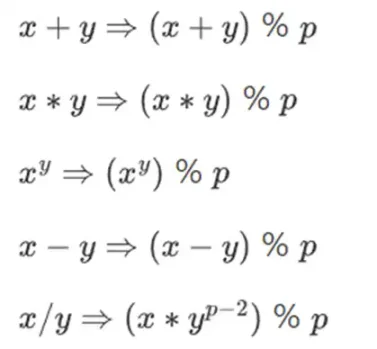
All of these rules are consistent. For example, if p=7, then:

5+3=1 (because 8%7=1)

1-3=5 (because -2%7=5)

2*5=3

3/5=2

A more general term for this structure is a finite field. A finite field is a mathematical structure that follows the usual arithmetic rules, but with a limited number of possible values, so each value can be represented with a fixed size.

Modular arithmetic (or prime fields) is the most common type of finite field, but there is also another type: extension fields. You may have seen an extension field: complex numbers. We "imagine" a new element, label it as i, and perform mathematical operations with it: (3i+2)*(2i+4)=6i*i+12i+4i+8=16i+2. We can also take extensions of prime fields. When dealing with smaller fields, extensions of prime fields become increasingly important for security, and binary fields (used by Binius) rely entirely on extensions to have practical utility.

Review: Arithmeticization

The method of proving computer programs in SNARK and STARK is through arithmetic: you convert a statement about the program you want to prove into a mathematical equation containing polynomials. The effective solutions of the equations correspond to the valid execution of the program.

For a simple example, suppose I calculated the 100th Fibonacci number, and I want to prove to you what it is. I create a polynomial F encoding the Fibonacci sequence: so F(0)=F(1)=1, F(2)=2, F(3)=3, F(4)=5, and so on, up to 100 steps. The condition I need to prove is F(x+2)=F(x)+F(x+1) for the entire range x={0,1…98}. I can convince you by providing a quotient:

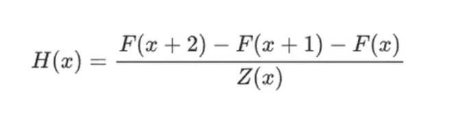
Where Z(x) = (x-0) * (x-1) * …(x-98). If I can provide an F and H that satisfy this equation, then F must satisfy F(x+2)-F(x+1)-F(x) within that range. If I also verify that F satisfies F(0)=F(1)=1, then F(100) must actually be the 100th Fibonacci number.

If you want to prove something more complex, then you replace the "simple" relationship F(x+2) = F(x) + F(x+1) with a more complex equation, which basically says "F(x+1) is the output of initializing a virtual machine, with state F(x)", and running a computation step. You can also replace the number 100 with a larger number, for example, 100000000, to accommodate more steps.

All SNARK and STARK are based on this idea, that is, using simple equations (sometimes vectors and matrices) on polynomials to represent a large number of relationships between individual values. Not all algorithms check the equivalence between adjacent computation steps like the example above: for example, PLONK and R1CS do not. But many of the most effective checks do, as performing the same check (or a small number of checks) multiple times can more easily minimize the overhead.

Plonky2: From 256-bit SNARK and STARK to 64-bit… only STARK

Five years ago, a reasonable summary of different types of zero-knowledge proofs is as follows. There are two types of proofs: (based on elliptic curves) SNARK and (based on hashes) STARK. Technically, STARK is a type of SNARK, but in practice, "SNARK" is usually used to refer to variants based on elliptic curves, while "STARK" is used to refer to structures based on hashes. SNARKs are small, so you can verify them very quickly and easily install them on the chain. STARKs are large, but they do not require trusted setups, and they are resistant to quantum attacks.

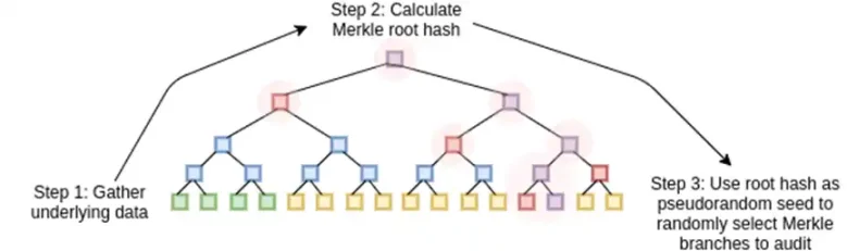
The working principle of STARK is to view the data as a polynomial, compute the polynomial, and use the Merkle root of the extended data as the "polynomial commitment".

One key historical point here is that SNARK based on elliptic curves first gained widespread use: it wasn't until around 2018 that STARK became efficient enough, thanks to FRI, and by then Zcash had been running for over a year. One key limitation of SNARK based on elliptic curves is that if you want to use SNARK based on elliptic curves, the arithmetic in these equations must be done using the point numbers modulo on the elliptic curve. This is a large number, usually close to 2^256: for example, the bn128 curve is 21888242871839275222246405745257275088548364400416034343698204186575808495617. But the actual calculations use small numbers: if you consider a "real" program in your favorite language, most of what it uses are counters, indices in for loops, positions in the program, single bits representing True or False, and other things that are almost always only a few digits long.

Even if your "original" data consists of "small" numbers, the proof process requires calculations of quotients, extensions, random linear combinations, and other data transformations, which will result in an equal or larger number of objects, the average size of which is as large as the entire size of your field. This leads to a key inefficiency: to prove calculations on n small values, you must perform more calculations on n much larger values. Initially, STARK inherited the habit of using a 256-bit field from SNARK, and therefore suffered from the same inefficiency.

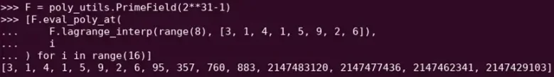
Reed-Solomon extension of some polynomial evaluations. Despite the original values being small, the additional values are extended to the full size of the field (in this case, 2^31 - 1).

In 2022, Plonky2 was released. The main innovation of Plonky2 is arithmetic modulo a smaller prime number: 2^64 - 2^32 + 1 = 18446744067414584321. Now, each addition or multiplication can always be completed in a few instructions on the CPU, and the speed of hashing all data together is four times faster than before. But there is a problem: this method only applies to STARK. If you try to use SNARK, the elliptic curve for such a small prime number will become insecure.

To ensure security, Plonky2 also needs to introduce extension fields. One key technique for checking arithmetic equations is "random point sampling": if you want to check if H(x) * Z(x) equals F(x+2)-F(x+1)-F(x), you can randomly select a coordinate r, provide a proof by committing to the polynomials H(r), Z(r), F(r), F(r+1), and F(r+2), and then verify if H(r) * Z(r) equals F(r+2)-F(r+1)-F(r). If an attacker can guess the coordinate in advance, the attacker can deceive the proof system—this is why the proof system must be random. But this also means that the coordinates must be sampled from a large enough set to prevent the attacker from guessing randomly. This is obviously the case if the modulus is close to 2^256. However, for a modulus of 2^64 - 2^32 + 1, we are not there yet, and if we reduce it to 2^31 - 1, the situation is definitely not the same. Trying to forge a proof 2 billion times until someone gets lucky is definitely within the capabilities of an attacker.

To prevent this situation, we sample r from the extension field, for example, you can define y, where y^3=5, and use combinations of 1, y, and y^2. This will increase the total number of coordinates to about 2^93. Most of the polynomials computed by the prover do not enter this extension field; they are only taken modulo 2^31 - 1, so you can still get all the efficiency from using the small field. But random point checks and FRI calculations do delve into this larger field to achieve the required security.

From Small Primes to Binary

Computers perform arithmetic operations by representing larger numbers as sequences of 0s and 1s, and building "circuits" on these bits to perform operations such as addition and multiplication. Computers are optimized for 16-bit, 32-bit, and 64-bit integers. For example, 2^64 - 2^32 + 1 and 2^31 - 1 are chosen not only because they meet these boundaries, but also because they are very close to these boundaries: multiplication modulo 2^64 - 2^32 + 1 can be performed by regular 32-bit multiplication, with some bit shifting and copying outputs in a few places; this article explains some tricks very well.

However, a better approach is to perform calculations directly in binary. What if addition can "simply" be XOR, without worrying about "carrying" from one bit adding 1 + 1 to the next bit? What if multiplication can be similarly parallelized? These advantages are all based on being able to represent true/false values with a single bit.

The advantages of being able to perform calculations directly in binary are exactly what Binius is trying to achieve. The Binius team demonstrated efficiency improvements at the zkSummit:

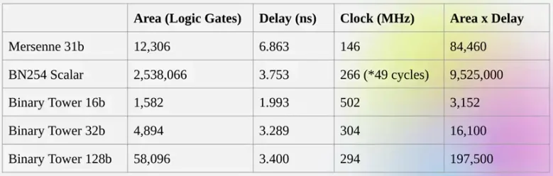
Although the "sizes" are roughly the same, operations on 32-bit binary fields require 5 times fewer computational resources than operations on 31-bit Mersenne fields.

From Univariate Polynomials to Hypercubes

Suppose we believe this reasoning and want to do everything with bits (0 and 1). How do we represent a billion bits with a polynomial?

Here, we face two practical problems:

1. For a polynomial representing a large number of values, these values need to be accessible during the evaluation of the polynomial: in the Fibonacci example above, F(0), F(1) … F(100), in a larger computation, the exponent would reach into the millions. The field we use needs to contain numbers up to this size.

2. Any value we submit in a Merkle tree (like all STARKs) needs to be Reed-Solomon encoded: for example, extending values from n to 8n, using redundancy to prevent a malicious prover from cheating by forging a value during the computation. This also requires a field large enough: to extend one million values to eight million, you need 8 million different points to compute the polynomial.

A key idea of Binius is to address these two problems separately and achieve the same data representation in two different ways. First, the polynomial itself. Systems like SNARK based on elliptic curves, STARK in the 2019 era, and Plonky2 typically deal with a univariate polynomial: F(x). On the other hand, Binius takes inspiration from the Spartan protocol and uses multivariate polynomials: F(x1, x2, … xk). In fact, we represent the entire computation trace on a "hypercube," where each xi is either 0 or 1. For example, if we want to represent a Fibonacci sequence and still use a field large enough to represent them, we can imagine the first 16 numbers like this:

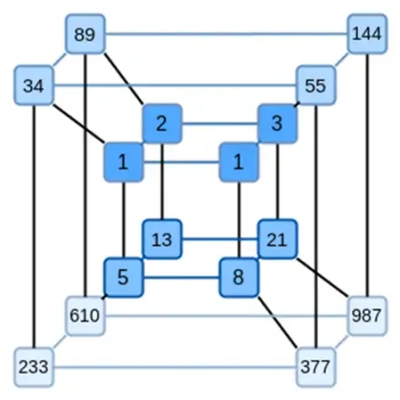
In other words, F(0,0,0,0) should be 1, F(1,0,0,0) should also be 1, F(0,1,0,0) is 2, and so on, all the way up to F(1,1,1,1)=987. Given such a computation hypercube, there will be a multivariate linear (degree 1 in each variable) polynomial that generates these computations. So we can think of this set of values as a representation of the polynomial; we don't need to compute the coefficients.

Of course, this example is just for illustration: in practice, the whole point of entering the hypercube is to allow us to work with individual bits. The "native" Binius way of computing Fibonacci numbers is to use a high-dimensional hypercube, with each group of, say, 16 bits representing a number. This requires some cleverness to perform integer addition based on bits, but for Binius, it's not too difficult.

Now, let's look at Reed-Solomon codes. The way STARK works is: you take n values, Reed-Solomon extends them to more values (usually 8n, typically between 2n and 32n), then randomly select some Merkle branches from the extension and perform some checks on them. The length of the hypercube in each dimension is 2. Therefore, directly extending it is impractical: there isn't enough "space" to sample Merkle branches from 16 values. So what do we do? We assume the hypercube is a square!

Simple Binius - An Example

Refer to the python implementation of this protocol here.

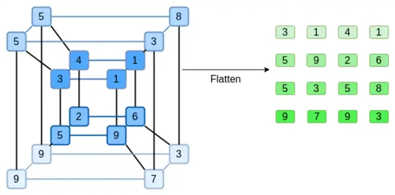
Let's look at an example, using regular integers as our field for simplicity (in actual implementation, binary field elements will be used). First, we encode the hypercube we want to submit as a square:

Now, we extend the square using Reed-Solomon. That is, we treat each row as a 3rd degree polynomial evaluated at x={0,1,2,3}, and the same polynomial evaluated at x={4,5,6,7}:

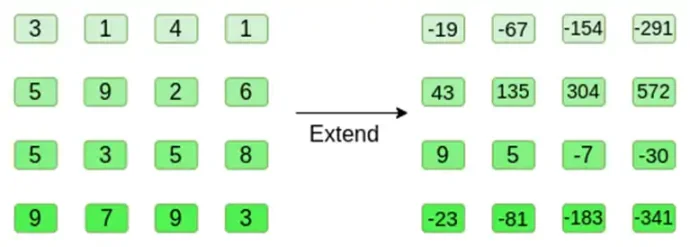
Note that the numbers quickly expand! This is why in actual implementation, we always use finite fields instead of regular integers: if we use integers modulo 11, for example, the extension of the first row would be [3,10,0,6].

If you want to try extending and verifying the numbers here yourself, you can use my simple Reed-Solomon extension code here.

Next, we treat this extension as columns and create a Merkle tree of the columns. The root of the Merkle tree is our commitment.

Now, let's say the prover wants to prove the computation of this polynomial at some point r={r0,r1,r2,r3}. There's a subtle difference in Binius that makes it weaker than other polynomial commitment schemes: the prover should not know or be able to guess s before submitting to the Merkle root (in other words, r should be a pseudorandom value dependent on the Merkle root). This makes the scheme useless for "database lookups" (e.g., "Okay, you gave me the Merkle root, now prove to me P(0,0,1,0)!"). But the zero-knowledge proof protocols we actually use typically don't require "database lookups"; they only need to check the polynomial at a random evaluation point. So, this limitation serves our purpose.

Let's say we choose r={1,2,3,4} (at which point the computation of the polynomial results in -137; you can confirm this using this code). Now, we enter the proof process. We split r into two parts: the first part {1,2} represents a linear combination within the columns, and the second part {3,4} represents a linear combination within the rows. We compute a "tensor product" for the column part:

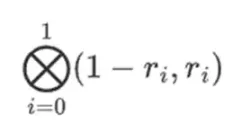
And for the row part:

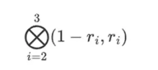
This means: a list of all possible products of one value from each set. In the row case, we get:

[(1-r2)(1-r3), (1-r3), (1-r2)r3, r2*r3]

Using r={1,2,3,4} (so r2=3 and r3=4):

[(1-3)(1-4), 3(1-4),(1-3)4,34] = [6, -9 -8 -12]

Now, we calculate a new "row" t by taking a linear combination of the existing rows. That is, we take:

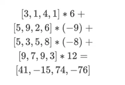
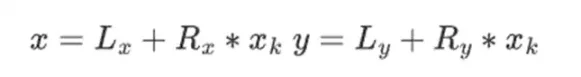
You can think of what happens here as partial evaluations. If we take the full tensor product and multiply by the full vector of values, you will get the computation P(1,2,3,4) = -137. Here, we will only use the partial tensor product of the evaluation coordinates and simplify the N-value grid to a row of square root N values. If you provide this row to someone else, they can use the tensor product of the other half of the evaluation coordinates to complete the remaining computation.

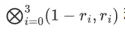
The prover provides the following new row to the verifier: t and a Merkle proof for some randomly sampled columns. In our illustrative example, we will have the proof process only provide the last column; in real life, the prover needs to provide several columns to achieve sufficient security.

Now, we use the linearity of the Reed-Solomon code. The key property we use is: taking a linear combination of a Reed-Solomon extension yields the same result as the extension of the linear combination. This "order independence" typically happens when both operations are linear.

This is exactly what the verifier does. They calculate t, and compute the linear combination of the same columns the prover previously computed (but only compute the columns the prover provided), and verify if these two processes yield the same answer.

In this example, we extend t and compute the same linear combination ([6,-9,-8,12]), and both yield the same answer: -10746. This proves that the Merkle root is "well-behaved" (or at least "close enough"), and it matches t: at least the majority of the columns are mutually compatible.

But the verifier still needs to check one more thing: the evaluation of the polynomial {r0…r3}. So far, all the verifier's steps have not actually depended on the values claimed by the prover. We check this by taking the tensor product of the "column part" we labeled as the evaluation point:

In our example, where r={1,2,3,4}, so the chosen half of the columns is {1,2}), which equals:

Now we take this linear combination t:

And this is the same as directly evaluating the polynomial.

The above content is very close to a complete description of the "simple" Binius protocol. It already has some interesting advantages: for example, since the data is split into rows and columns, you only need a field that's half the size. However, this doesn't achieve all the benefits of computing with binary. For that, we need the full Binius protocol. But first, let's delve deeper into binary fields.

Binary Fields

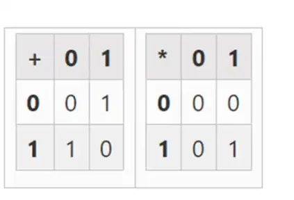
The smallest possible field is arithmetic modulo 2, which is very small, and we can write its addition and multiplication tables:

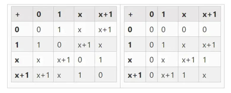
We can extend to larger binary fields by defining x where x^2=x+1, starting from F2 (integers modulo 2), and then we get the following addition and multiplication tables:

In fact, we can extend binary fields to any size by repeating this construction. Unlike complex numbers over real numbers, where you can add a new element but can't add any more elements (quaternions do exist, but they're mathematically weird, e.g., ab doesn't equal ba), with finite fields, you can keep adding new extensions forever. Specifically, we define elements as follows:

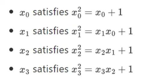
And so on… This is often called a tower structure, because each successive extension can be seen as adding a new layer to the tower. This isn't the only way to construct arbitrary-sized binary fields, but it has some unique advantages that Binius leverages.

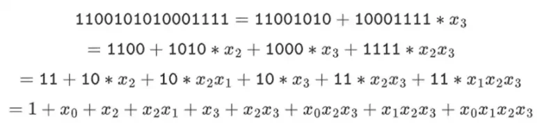
We can represent these numbers as a list of bits. For example, 1100101010001111. The first bit represents multiples of 1, the second bit represents multiples of x0, and the subsequent bits represent multiples of the following x1 numbers: x1, x1x0, x2, x2x0, and so on. This encoding is nice because you can factorize it:

This is a relatively uncommon representation, but I like to represent binary field elements as integers, with the more significant bits on the right. That is, 1=1, x0=01=2, 1+x0=11=3, 1+x0+x2=11001000=19, and so on. In this expression, it is 61779.

Addition in binary fields is just XOR (by the way, subtraction is also the same); note that this means x+x=0 for any x. Multiplying two elements x*y has a very simple recursive algorithm: split each number in half:

Then, split the multiplication:

The last part is the only slightly tricky part, as you have to apply simplification rules. There are more efficient ways to do multiplication, similar to the Karatsuba algorithm and fast Fourier transform, but I'll leave that as an exercise for interested readers to figure out.

Division in binary fields is done by combining multiplication and inversion. The "simple but slow" inversion method is an application of the generalized Fermat's little theorem. There's also a more complex but more efficient inversion algorithm, which you can find here. You can play with addition, multiplication, and division in binary fields using the code here.

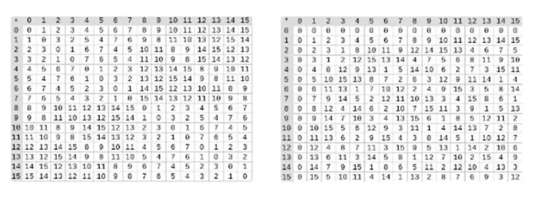
Left image: Addition table for four-bit binary field elements (i.e., consisting only of 1, x0, x1, x0x1). Right image: Multiplication table for four-bit binary field elements.

The beauty of this type of binary field is that it combines some of the best parts of "regular" integers and modulo arithmetic. Like regular integers, binary field elements are unbounded: you can extend them as you please. But like modulo arithmetic, if you operate on values within a certain size limit, all your results also stay within the same range. For example, if you take 42 to consecutive powers, you get:

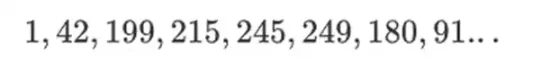
After 255 steps, you're back to 42 to the power of 255=1, just like with regular integers and modulo arithmetic, they follow the usual mathematical laws: ab=ba, a(b+c)=ab+a*c, and even some strange new laws.

Finally, binary fields can conveniently handle bits: if you perform mathematical operations with numbers that are powers of 2, all your outputs will also fit into powers of 2 bits. This avoids awkwardness. In Ethereum's EIP-4844, the various "blocks" of a blob must be numbers modulo 52435875175126190479447740508185965837690552500527637822603658699938581184513, so encoding binary data requires discarding some space and performing additional checks at the application layer to ensure that each element's stored value is less than 2 to the power of 248. This also means that binary field operations are super fast on computers—whether it's CPU, or theoretically optimal FPGA and ASIC designs.

All of this means that we can do what we did with Reed-Solomon encoding, in a way that completely avoids integer "explosions," as we saw in our example, and in a very "native" way, the kind of computation computers are good at. The "splitting" property of binary fields—how we split 1100101010001111 into 11001010+10001111*x3, and then split as needed—is crucial for achieving great flexibility.

Full Binius

Please refer to this python implementation of the protocol.

Now, we can move on to "Full Binius," which adjusts the "Simple Binius" to (i) work on binary fields, and (ii) allow us to submit individual bits. This protocol is difficult to understand because it switches back and forth between different ways of looking at the bit matrix; it took me longer to understand it than I usually spend understanding cryptographic protocols. But once you understand binary fields, the good news is that the "harder math" that Binius relies on doesn't exist. It's not elliptic curve pairings, where there are deeper and deeper algebraic rabbit holes to go down; here, you just need binary fields.

Let's take another look at the complete chart:

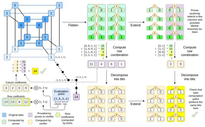
By now, you should be familiar with most of the components. The idea of "flattening" the hypercube into a grid, the idea of computing row combinations and column combinations as the tensor product of evaluation points, and the idea of checking the equivalence between "Reed-Solomon extension followed by row combination" and "row combination followed by Reed-Solomon extension" are all implemented in Simple Binius.

What's new in "Full Binius"? Basically, there are three things:

• Individual values in the hypercube and square must be bits (0 or 1).
• The extension process expands bits into more bits by grouping them into columns and temporarily assuming they are larger field elements.
• After the row combination step, there is an element-wise "decomposition into bits" step that converts the extension back into bits.

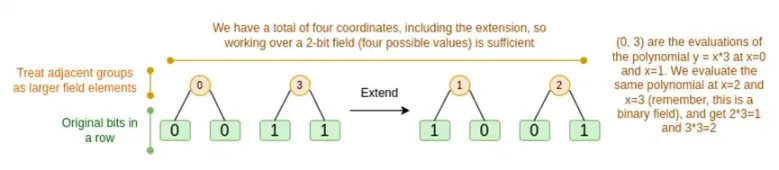
We will discuss these two cases in turn. First, the new deferred procedure. The Reed-Solomon code has a fundamental limitation: if you want to expand n to kn, you need to work in a field with kn different values that can be used as coordinates. This can't be done with F2 (also known as bits). So what we do is, we "pack" adjacent F2 elements together to form larger values. In the example here, we pack two bits at a time into {0,1,2,3} elements, because our extension only has four evaluation points, which is enough for us. In a "real" proof, we might return 16 bits at a time. Then, we apply the Reed-Solomon code to these packed values and then unpack them back into bits.

Now, the row combination. To check the encryption security of "evaluating at random points," we need to sample that point from a fairly large space (much larger than the hypercube itself). So while the points inside the hypercube are bits, the computed values outside the hypercube will be much larger. In the example above, the "row combination" ends up being [11,4,6,1].

Here's the problem: we know how to combine bits into a larger value and then perform a Reed-Solomon extension on that, but how do we do the same thing for larger values?

The trick of Binius is to work with bits: we look at the individual bits of each value (e.g., for something we label as "11," i.e., [1,1,0,1]), and then expand them row-wise. The expansion process is performed on the object. That is, we perform the extension process on each element's 1 row, then on the x0 row, then on the "x1" row, then on the x0x1 row, and so on (well, in our toy example, we stop there, but in the actual implementation, we will reach 128 rows (the last one being x6…x0)).

Recap:

• We convert the bits in the hypercube into a grid
• Then, we view adjacent bits on each row as larger field elements and perform arithmetic operations on them to Reed-Solomon extend the rows
• Then, we take the row combination of each column of bits and get the bit columns of each row as the output (much smaller for squares larger than 4x4)
• Then, we view the output as a matrix and then its bits as rows

Why do it this way? In "ordinary" mathematics, if you start slicing a number into bits, the ability to perform linear operations in any order and get the same result (usually) fails. For example, if I start with the number 345, multiply it by 8, and then multiply it by 3, I get 8280, and if I reverse these two operations, I also get 8280. But if I insert a "bitwise split" operation between the two steps, it breaks down: if you do 8 times, then 3 times, you get:

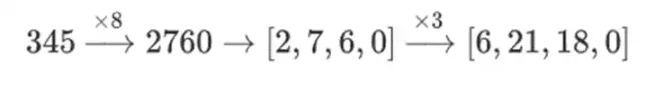
But if you do 3 times, then 8 times, you get:

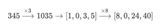
However, in binary fields constructed with a tower structure, this method does work. The reason is their separability: what happens on each segment when you multiply a large value by a small value stays on each segment. If we multiply 1100101010001111 by 11, this is the same as the first time we split 1100101010001111, resulting in:

Then each component is multiplied by 11.

Generally, the working principle of zero-knowledge proof systems is to make statements about polynomials while also representing statements about the underlying evaluations: just like we saw in the Fibonacci example, F(X+2)-F(X+1)-F(X) = Z(X)*H(X) checks all the steps of the Fibonacci calculation. We check statements about polynomials by proving evaluations at random points. This random point check represents a check of the entire polynomial: if the polynomial equation doesn't match, the likelihood of it matching at a specific random coordinate is very low.

In practice, one major reason for inefficiency is that most of the numbers we deal with in actual programs are very small: indices in for loops, True/False values, counters, and similar things. However, when we use Reed-Solomon encoding to "extend" data to provide the redundancy required for secure Merkle proof checks, most of the "extra" values end up taking up the entire size of the field, even if the original values are very small.

To address this issue, we want the field to be as small as possible. Plonky2 brought us down from 256-bit numbers to 64-bit numbers, and then Plonky3 further reduced it to 31 bits. But even this is not optimal. With binary fields, we can handle individual bits. This makes the encoding "dense": if your actual underlying data has n bits, then your encoding will have n bits, the extension will have 8*n bits, with no extra overhead.

Now, let's take a third look at this chart:

In Binius, we focus on a multilinear polynomial: a hypercube P(x0,x1,…xk), where individual evaluations P(0,0,0,0), P(0,0,0,1) up to P(1,1,1,1) store the data we care about. To prove a calculation at a certain point, we "reinterpret" the same data as a square. Then, we extend each row using Reed-Solomon encoding to provide the necessary data redundancy for random Merkle branch queries. Then we compute a random linear combination of rows, design coefficients to make the new combined row actually contain the values we care about. This newly created row (reinterpreted as 128 rows of bits) and some randomly selected columns with Merkle branches are passed to the verifier.

The verifier then performs "extended row combination" (or more precisely, extended columns) and "row combination extension," and verifies if they match. Then a column combination is computed and checked if it returns the value declared by the prover. This is our proof system (or more precisely, a polynomial commitment scheme, which is a key component of the proof system).

What haven't we talked about?

• Efficient algorithms for extending rows, which are necessary to actually improve the efficiency of verifier computation. We use fast Fourier transform on binary fields, as described here (although the exact implementation will be different, as this article uses a less efficient structure not based on recursive extension).
• Arithmeticization. Univariate polynomials are convenient because you can do things like linking adjacent steps in a calculation, such as F(X+2)-F(X+1)-F(X) = Z(X)*H(X). In the hypercube, the interpretation of "the next step" is far less clear than "X+1." You can do X+k, k powers, but this jumping behavior sacrifices many key advantages of Binius. The Binius paper introduces a solution (see section 4.3), but this itself is a "deep rabbit hole."
• How to securely perform specific value checks. The Fibonacci example requires checking critical boundary conditions: F(0)=F(1)=1 and the value of F(100). But for the "original" Binius, checking at known computations points is insecure. There are fairly simple ways to transform known computation checks into unknown computation checks, using so-called sum-check protocols, but we haven't discussed those here.
• Look-up protocols, another recently widely used technique used to make ultra-efficient proof systems. Binius can be combined with look-up protocols for many applications.
• Beyond square root verification time. Square roots are expensive: a Binius proof for 2 to the power of 32 bits is about 11MB long. You can use other proof systems to address this issue, to make "proofs of Binius proofs," achieving the efficiency and smaller proof size of Binius proofs. Another option is the more complex FRI-binius protocol, which creates a proof of logarithmic size (like regular FRI).
• How Binius affects "SNARK-friendliness." The basic summary is that if you use Binius, you no longer need to worry about making computations "arithmetic-friendly": "regular" hashes are no more efficient than traditional arithmetic hashes, multiplication modulo 2 to the power of 32 or modulo 2 to the power of 256 is no longer a headache compared to arithmetic multiplication, and so on. But this is a complex topic. Many things change when everything is done in binary form.

I hope that in the coming months, there will be more improvements in proof technology based on binary fields.

免责声明：本文章仅代表作者个人观点，不代表本平台的立场和观点。本文章仅供信息分享，不构成对任何人的任何投资建议。用户与作者之间的任何争议，与本平台无关。如网页中刊载的文章或图片涉及侵权，请提供相关的权利证明和身份证明发送邮件到support@aicoin.com，本平台相关工作人员将会进行核查。