2026-11-06 · Overseas Market Strategy · Event Commentary

Core Views

This sharp decline is primarily triggered by a concentrated sell-off due to deleveraging. The QQQ fell 6.49% in a single day, closing at 647.05, with the trading volume approximately 3.03 times the average of the previous 20 days. Historically, rebounds after such sharp drops are not uncommon; whether it can recover half of the decline within 60 trading days is the dividing line between a one-time shock and the start of a bear market.

In the short term, focus is on volatility recovery; in the long term, it depends on 2027 earnings. In the next one to two months, there is a high probability of another retracement around the FOMC in mid-December and the Texas ERCOT audit results. Long-term, whether the AI bubble will burst depends on whether 2027 earnings expectations are significantly revised down; if earnings downgrades and valuation compressions occur simultaneously, predictions must follow the trajectory of the 2000 tech bubble.

The end of the text provides entry and exit rules for both rebound and wait-and-see strategies, which is merely logical reasoning and does not constitute operational advice.

1. The sharp decline was triggered by deleveraging, with policy costs as the mid-term variable

QQQ closed at the lowest point of the day on November 5, about 4.94% below the 200-day moving average. Meanwhile, the 50-day moving average remains at 722.27, above the 200-day moving average of 680.71, indicating that the long-term moving averages have not yet formed a dead cross, but the price has clearly lost its trend support. This combination resembles the early phase of a trend reversal; simply relying on moving averages still pointing upwards is insufficient to conclude that the adjustment has ended.

The main line of this sell-off is the construction of AI data centers, and after the mid-term elections, market expectations regarding regulation have changed, leading to a reevaluation of project approvals, electricity costs, and construction cycles. According to institutional interpretations of the elections, state-level policies may further differentiate data center construction in the U.S., with political changes in Texas particularly likely to lengthen project timelines.

The amplification effect in trading has quite clear quantitative clues this time. According to estimates from several major brokerages, the rebalancing sell-offs of leveraged ETFs before the market close on November 5 were between $47 billion to $60 billion, compounded by passive sell-offs following CTA trend strategies exceeding $70 billion. This scale ranks second only to the record $51 billion to $55 billion on June 5 of this year.

The rebalancing of leveraged ETFs was essentially completed before that day’s close. After this round of deleveraging, the implied short gamma exposure has dropped from about $7.5 billion per 1% movement to around $6.5 billion, and subsequent passive sell-offs triggered by equivalent declines will correspondingly decrease. The volatility target strategy, which may last several days, still has about $50 billion of stock exposure that needs to be sold off in the coming days, as the target leverage drops from a historical 67% percentile to the 30% percentile.

The hedging purchases on November 5 indeed pressed yields lower, with the 2-year Treasury yield declining about 11 basis points to 4.46%, the lowest since September 10, while the 10-year yield dropped from 4.90% to 4.84%, marking a two-month low. However, viewed over a longer window, the 10-year yield reached as high as 5.365% in early October, the highest since 2002, and remains about 76 basis points higher than a year ago, with the 30-year yield also hovering around 5.26%. The short-end drop reflects safe-haven demand and adjustments in interest rate expectations, while the long-end still bears inflation and fiscal premiums; mid-term financing conditions remain to be improved.

2. Rebounds after sharp declines are not rare; whether half of the decline can be recovered is the watershed

Looking back at 13 representative sharp declines since 1987, 12 saw gains the following day.

Even in sustained bear markets, large gains the next day are quite common. Following a sharp drop on April 14, 2000, the Nasdaq rebounded 6.56% the next day, and there was a 5.45% rebound after September 29, 2008. Strong rebounds indicate changes in bullish and bearish forces post sharp declines, but this alone cannot prove that the market has bottomed.

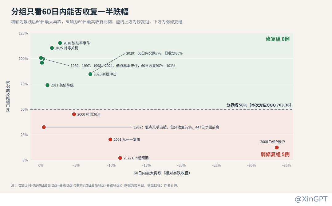
To compare different paths after sharp declines, we group these 13 sharp declines using a single rule: looking at whether the index can recover half of the decline from the prior high to the sharp decline close within 60 trading days. In the recovery group, those recovering over 50% within 60 days can be classified as one-off shocks within a bull market; conversely, the weak recovery group, with less than 50% recovery, indicates a bear trend beginning with the sharp decline.

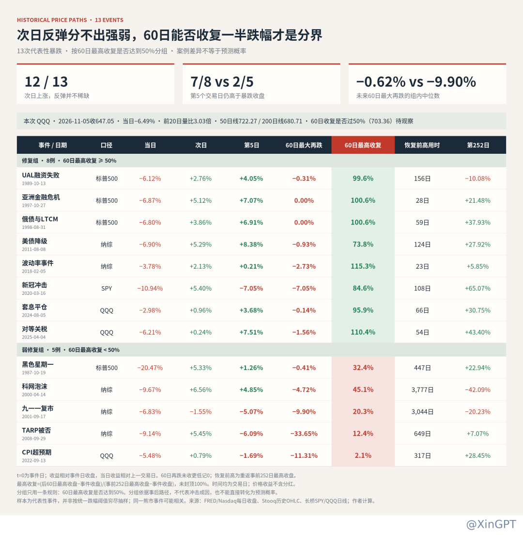
The differences between the two groups can be understood from three aspects.

First, whether the lows are held. In the recovery group, 7 out of 8 maintained a level above the sharp decline closing price on the 5th trading day, with a median further decline within 60 days of only 0.62%; of the weak recovery group’s 5 occurrences, only 2 managed this, with a median further drop reaching 9.90%, while in 2008, there was a further drop of over 30% within 60 days.

Secondly, how high the rebound can go. The median recovery ratio within 60 days in the recovery group is around 100%, essentially returning to near previous highs within two to three months; the weak recovery group’s median is only about 20%, where rebounds often face obstacles after recovering only 20% to 40% of the decline.

Finally, the results one year later. In the recovery group, 7 out of 8 saw a price increase after one year, with the only exception being 1989; the weak recovery group, however, shows divergence, with declines of 42% and 20% a year later in 2000 and 2001 respectively, continuing bear market trends, while in 1987, 2008, and 2022, the trend reversed to price increases after a year.

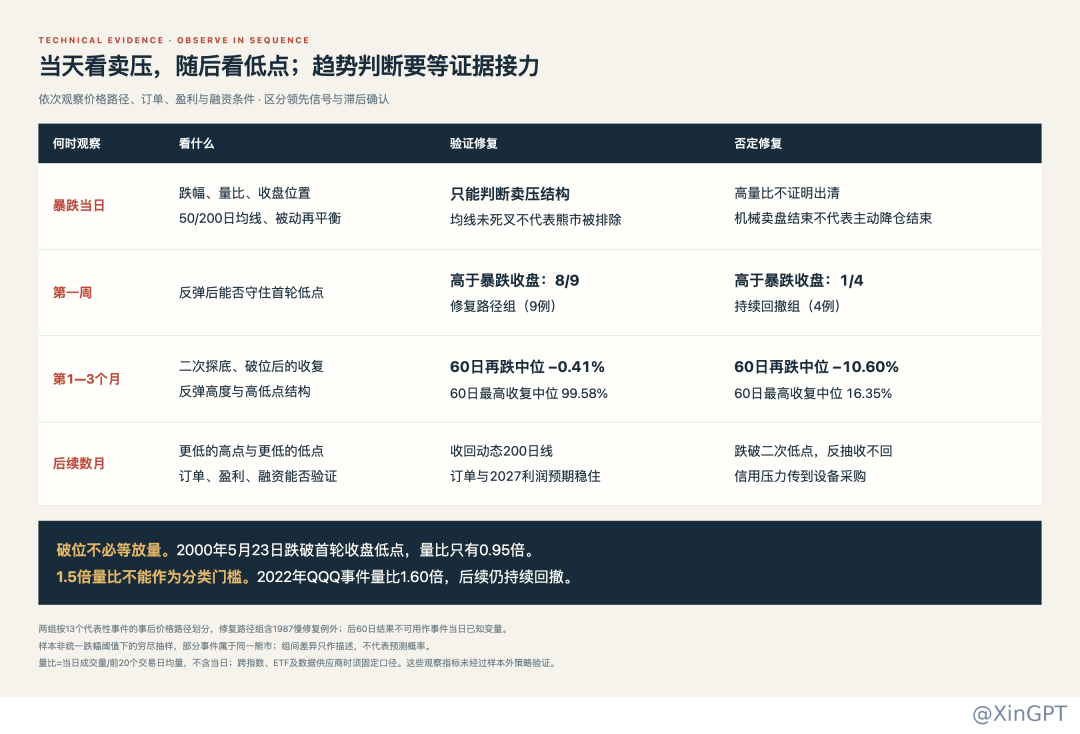
The path taken is determined by earnings and valuations; orders and financing will signal first

The above grouping only illustrates what happened after the sharp decline; regarding why different paths are taken, attention must return to the components of stock prices, which is earnings multiplied by valuations. Any issues in these two components can significantly determine subsequent trends, and both do not always move in the same direction.

During the pandemic in 2020, corporate profits fell significantly, yet policy support allowed the market to assign higher valuations, and stock prices rebounded first; in 2022, corporate earnings did not collapse, but the Fed’s rapid rate hikes drastically compressed valuations, leading the index to also enter bear market territory. Therefore, to ascertain which group this shock will belong to, one must observe both earnings and valuations, focusing on whether both will deteriorate simultaneously.

3. The lesson from 2000 is that rebounds can be significant while the trend remains downward

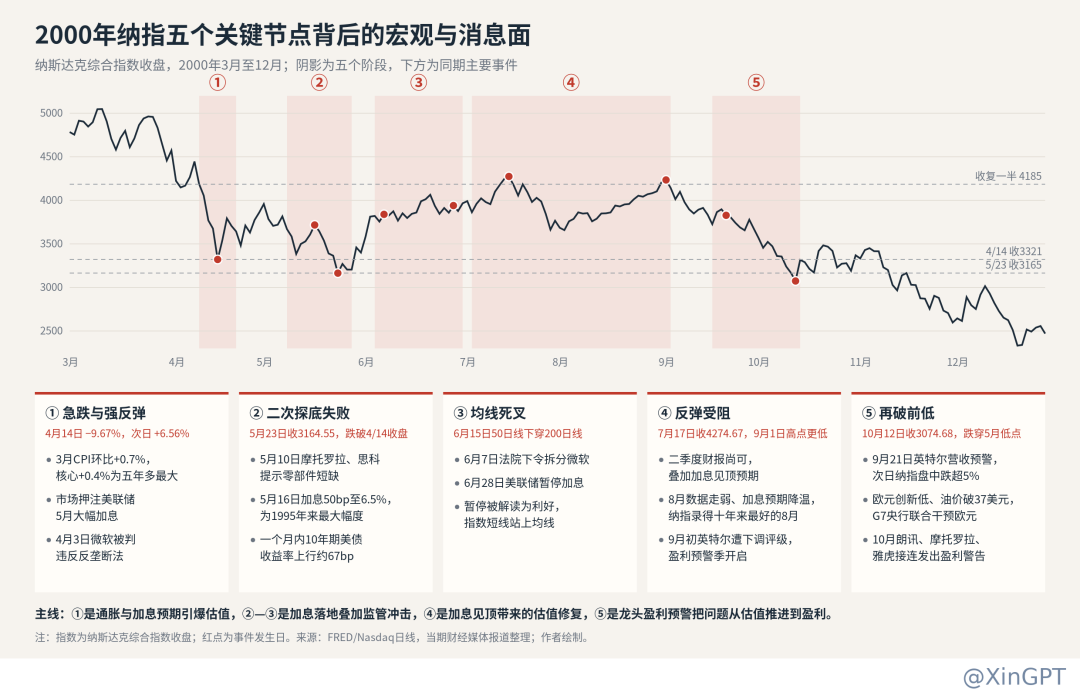
The reference value from 2000 lies in its comprehensive demonstration of how a bubble peak was gradually confirmed. On April 14, the Nasdaq plunged 9.67%, only to rebound 6.56% the next day and reclaim the 200-day moving average. However, it subsequently experienced failed attempts to retest the low, long-term moving averages forming a death cross, resistance encountered during rebounds, and renewed lows. A few months of price and fundamental validations separated the first rebound from an actual trend reversal.

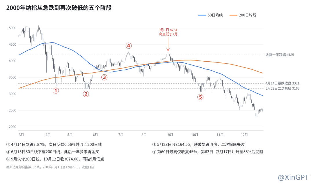
The first crack appeared during the second retest. The Nasdaq closed at 3321.29 on April 14, rebounded to 3958.08 on May 1, but fell back to 3164.55 on May 23, first breaking below the closing price on the day of the plunge. The previous rebound failed to form a higher low, thus negating the price recovery; furthermore, the volume on that day was only 0.95 times, indicating that a break did not require additional volume to confirm.

Next was the weakening of the moving average structure. On June 15, the 50-day moving average at 3688.75 crossed below the 200-day moving average at 3699.86. Interestingly, the index stood above both moving averages that day, indicating that the moving average crossover reflected pre-accumulated trend changes. It wasn’t until January 2002 that both moving averages registered a brief golden cross.

The third signal was a lack of strength in the bullish push. Using the highest close of 5048.62 on March 10 and the close of 3321.29 on April 14 as anchors, recovering half of the decline requires a return to 4184.96. By the 60th trading day on July 12, the highest close within that window was only 4099.59, recovering 45.06%; on July 17, which is the 63rd trading day, the index rose to 4274.67, achieving a recovery ratio of 55.19%, but it never managed to reclaim 60% of the decline.所谓弱修复，反而是反弹始终无法重新搭建起上升结构。

The definitive confirmation came from the loss of support for the moving averages and the preceding low being breached. The rebound high on September 1, 4234.33, was slightly below that of July 17, and on September 8, the index once again fell below the 200-day line, closing at 3074.68 on October 12, dropping below May’s close of 3164.55. These signals occurred sequentially over time and together were much more persuasive than the isolated occurrence of any one alone.

By comparing these five nodes against the macro and news backdrop at the time, the main line becomes clearer. The sharp decline was triggered by unexpectedly high inflation and interest rate expectations; the May rate hike plus the Microsoft breakup theme triggered a second round of declines. The Fed paused rate hikes in June and supported a summer rebound, but the true breaking point came after September when major companies like Intel and Lucent issued profit warnings. In other words, the issues of 2000 began with valuations and ultimately fell to earnings, which is precisely the scenario of simultaneous deterioration of earnings and valuations mentioned earlier.

The three thresholds in this price recovery

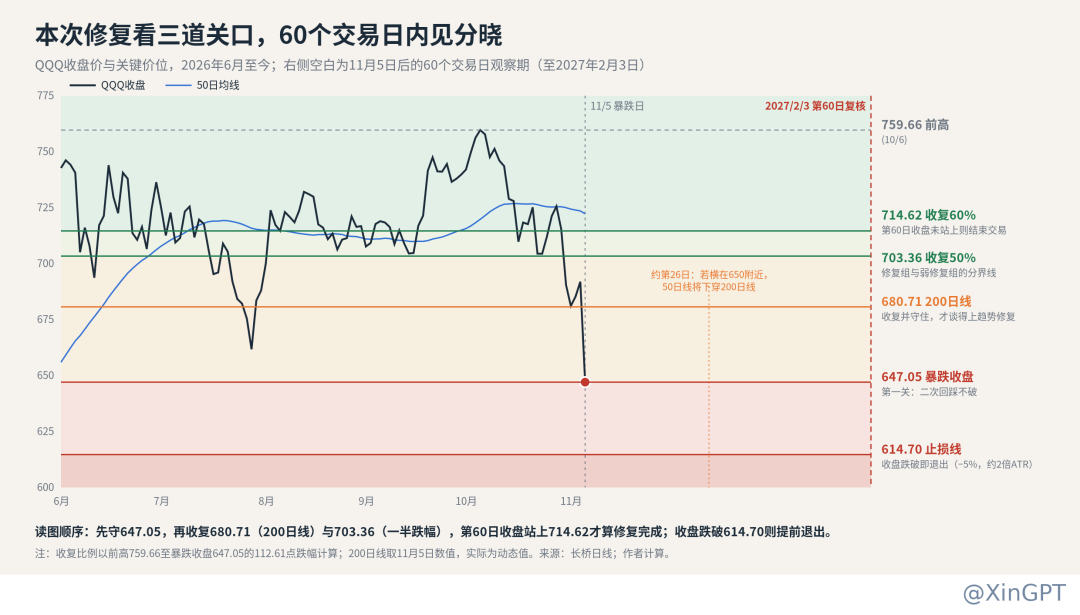
Using the same criteria, the QQQ fell from a previous high of 759.66 to 647.05, with half and sixty percent recoveries corresponding to 703.36 and 714.62. Recovery must surpass three thresholds: first, hold above 647.05; second, reclaim the 200-day line and 703.36; finally, on February 3, 2027, the 60th trading day, close above 714.62. Should the price linger around 650 for a long time, and if the 50-day line crosses below the 200-day line around the 26th trading day, the reference weight for the 2000 path will significantly increase. Current valuations being lower than in 2000 can buffer some risks, but as long as discount rates and risk premiums rise, valuations will still be compressed.

4. Fundamentals must be vigilant against profit expectation downgrades and valuation compressions

On the fundamentals level, two things need to be monitored: first, how much the index will be dragged down if 2027 profits are downgraded; second, whether such downgrades have shown early signs in the fourth-quarter data.

Impact of 2027 profit downgrades on the index

Analysis by Barclays strategists reveals that approximately 75% of the upward revisions to 2027 S&P profit forecasts during the year are driven by semiconductors and hardware. Therefore, the next question worth our attention is: If orders and pricing fall below expectations and performance is downgraded, how much will the index fall in tandem?

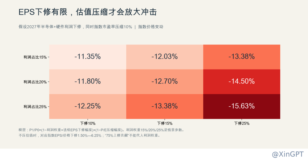
Calculating involves two steps. The first step calculates profits, taking FactSet's October 30 estimate of 2027 S&P EPS at 423.90 as a base, assuming the semiconductor and hardware segments account for a proportion of index profits w (using three tiers: 15%, 20%, 25%), and downgrading their profits d (using three tiers: 10%, 15%, 25%); if other industries remain unchanged, the index EPS drop equals w × d. The second step calculates valuation: the index level equals EPS multiplied by PE ratio, and if the PE ratio compresses p, the theoretical index drop is 1 − (1 − w×d) × (1 − p).

Simply looking at profits, the actual impact is limited. Taking the neutral scenario as an example, if the group accounts for 20% and downgrades by 15%, the index EPS drops from 423.90 to 411.18, a mere 3% decrease. But when compounded with valuation compression, the results vary dramatically, as shown in the table below with w fixed at 20%.

The conclusion is direct: profit downgrades alone will lead to single-digit declines, while for the index to drop by 20%, it relies primarily on simultaneous PE ratio compression.

Whether the PE ratio will compress mainly hinges on several points: firstly, interest rates; the 10-year U.S. Treasury yield is still above 4.8%, and there may be changes in market views regarding December's interest rate hikes and next year's yield curve; secondly, earnings visibility; if downgrades spread from semiconductors to vital weights in cloud computing, software, advertising, and consumer electronics, the market will assign a lower overall valuation to the index; thirdly, risk appetite; if corporate bond spreads widen, it indicates that the bond market is already pricing risks for AI investments, and equity investors will also require higher returns, leading to a decline in the PE ratio. Only simultaneous deterioration in all three areas will lead to the scenarios in the lower right corner of the table.

Q4 total earnings have not yet reversed, the first window for monitoring downgrades

Our judgment is that the probability of significant downgrades in Q4 earnings is low. As of October 30, only 40.4% of the 47 companies that issued Q4 guidance provided negative forecasts, which is significantly lower than the 60% five-year average. Analysts even adjusted their Q4 EPS predictions from 93.49 to 94.79 in October. The seven tech giants saw a Q3 earnings growth of 22.6%, although it was below the expected 33.6%, mainly due to investment losses and litigation costs, rather than operational deterioration.

Furthermore, even if there is a downgrade in Q4, the overall impact on the year will be limited. Calculating based on the full-year EPS of 363.94 in 2026 and 94.79 for Q4 yields the following.

Thus, the focus of the fundamentals is not on Q4, but on the earnings expectations for 2027. During the earnings season starting in late January, the real focus will be on companies' guidance for 2027. Once the 2027 S&P EPS consensus estimate of 423.90 begins to be revised down continuously, it will be necessary to reassess the downside capacity of the index in accordance with the tables in the previous section.

5. Credit stratification and tightening policies are two major external risks

Credit markets are already stratified, with weak entities seeing spreads widen first

AI capital expenditures are increasingly reliant on external financing, and the credit market is the first to reflect the pressure, and such differentiation has become very apparent. As of October 21, the five-year CDS for Oracle was reported at 331 basis points, Amazon at 80 basis points, and Microsoft at 56 basis points. In terms of cash flow, Microsoft’s operating cash flow of $58 billion in a single quarter is still sufficient to cover capital expenditures of $39.367 billion, while Amazon's free cash flow has decreased to –$42.357 billion over the past 12 months, and Alphabet also turned negative with a $9.1 billion loss in Q3.

The risks will initially stem from Oracle and new cloud companies reliant on external financing, while large platforms still have operational cash flows and credit that can be mobilized. We are tracking credit risk with the following three-tier rule, with the standards set for this article.

Policy risks are concentrated on grid costs and project licensing

After the mid-term elections, the focus of policy risk shifted from federal to state levels. The Democrats secured control of both houses, but Trump's veto power makes it difficult for national construction to be legislated, and rules such as requiring data centers to bear their own grid costs, along with Congressional investigations and hearings, are more likely to come into effect.

The real variable lies in Texas, which accounts for about a quarter of the U.S. capacity planned for 2030. The market previously expected the ERCOT audit, ordered by Abbott, to resume approvals after concluding in mid-December. However, newly elected Governor C inhibitionsa has proposed a total suspension of construction before legislation in the state legislature, coupled with the cancellation of tax incentives; upon taking office in January, she can extend the existing pause without new laws, leading to extended approval freezes. The state legislature, meeting simultaneously, will also engage in struggles over water use, electricity costs, and tax incentives.

The mainstream market judgment is one of delay, rather than cancellation; Texas will transition from a halt toward conditional re-authorization but at higher costs and without subsidies. Goldman Sachs estimates that states where Democrats could potentially tighten regulations cumulatively account for about 45% of planned capacity nationwide, while UBS estimates that about 30% of anticipated new capacity in 2028 may be affected, with approximately 18GW in Texas. Two key upcoming nodes are: first, after the mid-December ERCOT audit results, whether the new government will extend the pause; second, in January's earnings season, whether cloud companies provide guidance for 2027 capital expenditures. To date, no company has downgraded; once downgrades occur or Texas projects are shifted heavily to other states, it will mean a true turning point in policy.

6. Short-term volatility recovery depends on 2027 earnings in the long term

Short-term views

In the next one to two months, a preference for volatile recovery is noted. The passive sell-offs from leveraged ETFs are essentially cleared, and historically, most sharp declines are followed by decent rebounds, but the volatility target strategy of around $50 billion in sell-offs is still in progress; additionally, mid-December brings the potential for an FOMC rate hike plus ERCOT audit results, making it highly likely there will be a reassessment process around 647.05. The rebound target initially stands at 680.71 to 703.36, and the ability to break through these depends on January's earnings season.

Long-term views

We tend to believe this is a deceleration in the AI cycle rather than a peak. Compared to 2000, current profits are still being revised upwards, and valuations are also lower. The policy impacts primarily bring delay rather than cancellation; however, the similarity lies in that optimistic expectations for the index are highly concentrated among a few sectors, and the interest rate environment is less friendly than in 2000. If after January's earnings season, the consensus 2027 EPS estimate does not show significant downgrades, and credit spreads remain stable, it is more likely this will lead to a recovery group path, turning pullbacks into opportunities for mid- to long-term positioning; conversely, should downgrades and valuation compressions occur simultaneously, the approach must align with that of 2000, reducing positions and waiting for earnings to stabilize before re-entering.

7. Operational thoughts are for reference only

The following levels and directions are merely logical deductions based on earlier analyses, not constituting investment advice, and direct imitation is not recommended. Specific operations should align with personal risk preferences and position conditions.

Rebound or wait-and-see

The difference between the two approaches lies in how much uncertainty one is willing to bear. Engaging in a rebound means entering near 647.05 first, using about a 5% stop-loss to obtain a lower cost, suitable for investors who can strictly enforce exit discipline; while waiting means forgoing the initial rebound, waiting for the market to prove that the low is effective before entering, resulting in higher costs but potentially higher success rates, suited for those with heavier positions or who cannot withstand secondary lows.

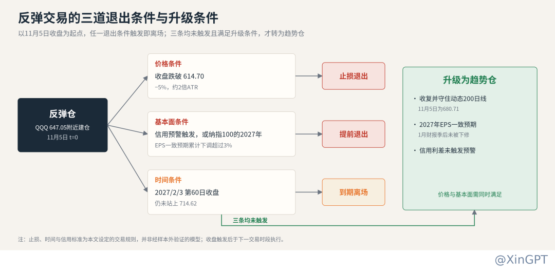
Positions in a rebound are treated purely based on rebound trading; there are three exit conditions, with any triggering leading to exit: a daily close below 614.70 for stop-loss; if credit warnings are triggered, or if the 2027 EPS consensus for the Nasdaq100 is revised down more than 3%, exit in anticipation of price signals; if the close on February 3, 2027, the 60th trading day, hasn't stood above 714.62, exit upon expiration. If none of these three are triggered and the price recovers and stays above the 200-day line, with no revisions to the 2027 earnings expectations, then upgrade the rebound position to a trend position.

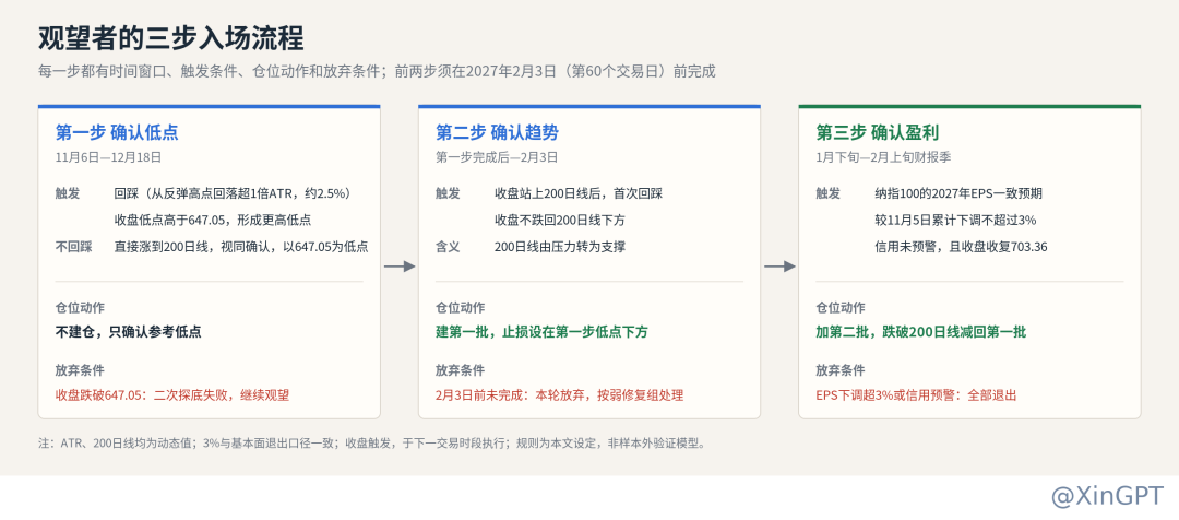
For those waiting to enter, it’s a three-step process, with timing and exit conditions for each step.

The first step is confirming the low, with a window until December 18, coinciding with both FOMC and ERCOT audit events. If QQQ falls back over one ATR (approximately 2.5%) from the rebound high, it’s treated as a retracement; only if the closing low of the retracement is higher than 647.05 can a higher low be confirmed; if there is no retracement and the price directly rises to the 200-day line, this is treated as confirmation, using 647.05 as the reference low; if it closes below 647.05, it signals a failed second bottom and continues waiting. No positions are built in this step.

The second step is confirming the trend, where the standard is that the 200-day line changes from resistance to support, that is, the first time it closes above the 200-day line and the first closed retracement does not fall below the line, at which point the first batch of positions is established, with stop-loss set below the reference low of the first step. If the first two steps are not completed by February 3, it suggests this corresponds closer to the weak recovery group, and participation in this round will cease.

The third step confirms profits, with the review date set for early February after the major weight companies like Microsoft, Meta, Apple, Amazon, and Google finish reporting earnings. If the 2027 EPS consensus for the Nasdaq100 does not fall more than 3% from the cumulative revisions on November 5, and there are no credit warnings, the fundamentals will provide a basis for increasing positions, where the condition is for the close to stand above 703.36. If it has already stood above this prior to the review confirmation, a second batch will be added after the review confirmation; if it has not yet stood above during the review, maintain only the first batch up to the first close above it for an add-on.

Stop-losses are set based on the "reason for building positions becoming invalid," applying individually for each batch. The first batch's reason is the confirmation of the low; if the close breaches the reference low, exit. The second batch's reason ties to the simultaneous confirmation of trend and profits, with the trend marked by the support of the second step's 200-day line, hence close falling back below the 200-day line triggers a sell-off of the second batch. Furthermore, regardless of the stage, if the cumulative EPS revisions exceed 3% or credit warnings are triggered, both batches will exit; this standard aligns perfectly with the fundamental exit conditions of the rebound positions.

Market observations are anchored on the close of November 5, 2026, and data is up to November 6, 2026, maintaining precise terms for price, earnings, and credit data as in the original text. Historical events are representative samples, and sector weightings, profit downgrades, valuation compressions, and trade triggers are all scenario assumptions or guidelines established in this article.

— — — — —

免责声明：本文章仅代表作者个人观点，不代表本平台的立场和观点。本文章仅供信息分享，不构成对任何人的任何投资建议。用户与作者之间的任何争议，与本平台无关。如网页中刊载的文章或图片涉及侵权，请提供相关的权利证明和身份证明发送邮件到[email protected]，本平台相关工作人员将会进行核查。