Original Title:Game Theory on Polymarket: The 5 Formulas tested on 72 million trades, Author: Movez (@0xMovez)

Translated by｜Odaily Stellar Daily (@OdailyChina); Translator｜Asher (@Asher_0210)

On the Las Vegas Strip, the average return rate on slot machines is about 93%, meaning for every dollar spent, players can expect to get back only $0.93; yet on Polymarket, traders willingly accept returns as low as $0.43, betting $1 on obscure outcomes with odds worse than those at a casino.

This is not a metaphor, but based on real data. Researcher Jonathan Becker conducted an analysis of all settled markets on Kalshi, covering 72 million trades and a total trading volume of $18.26 billion. The patterns he discovered also apply to Polymarket—same mechanisms, same biases, which also imply the same opportunities. The conclusion drawn from the data is straightforward: about 87% of prediction market wallets end up losing money, but the remaining 13% do not win by luck; they have mastered a set of mathematical techniques that most traders have not even understood.

This article will break down 5 game theory formulas that distinguish winners from losers, each accompanied by corresponding mathematical principles, real cases, and runnable Python code. Some traders who have already applied these methods in practice include:

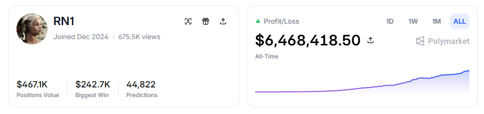
• RN (Polymarket address: https://polymarket.com/profile/%40rn1): An algorithmic trading bot on Polymarket, which realized over $6 million in total profits in sports markets based on the models in this article.

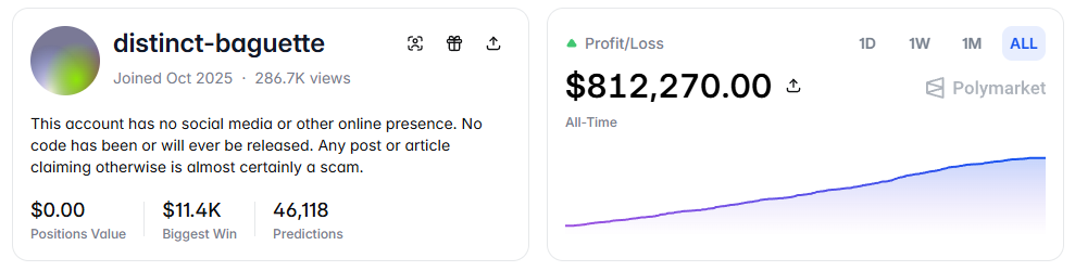
• distinct-baguette (Polymarket address: https://polymarket.com/profile/%40distinct-baguette): Rolled over $560 to $812,000 through market making in UP/DOWN markets.

1. Expected Value: The Core Formula

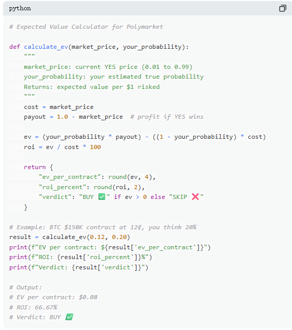
On Polymarket, each trade is essentially an expected value judgment. Most traders rely on intuition, while that 13% of winners make decisions based on mathematics. Expected value (EV) measures not the outcome of a single event, but the average return after multiple repetitions, used to assess whether a trade is worth participating in.

For example, in a real market, “Will Bitcoin reach $150,000 before June 2026?” The current YES price is $0.12, corresponding to an implied market probability of 12%. If based on on-chain data, halving cycles, and ETF capital flows, the real probability is assessed to be around 20%, then this trade has positive expected value. By this calculation, each contract bought at $0.12 could yield an average profit of $0.08 in the long run; buying 100 contracts, with a corresponding cost of $12, the expected profit would be $8, yielding a return rate of about +66.7%.

However, data shows that most prediction market traders do not conduct such calculations. In a sample covering 72 million trades, takers (market order buyers) have an average loss of about 1.12% per trade, while makers (those who place limit orders) have an average gain of about 1.12%. The gap between the two is not about information but patience—makers wait for opportunities with positive expected value, while takers are more prone to impulsive trading.

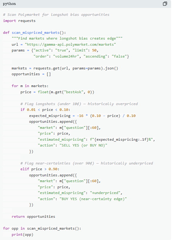
2. Mispricing: The Low Price Contract Trap

“Underdog preference” is one of the most expensive mistakes in prediction markets, where traders often systematically overestimate low-probability events, paying excessively high prices for what appear to be cheap contracts. A contract priced at $0.05 should theoretically have a 5% win rate, but the actual win rate on Kalshi is only 4.18%, corresponding to a pricing bias of -16.36%; in more extreme cases, a $0.01 contract is supposed to have a 1% win rate, but for takers, the actual win rate is only 0.43%, with a bias as high as -57%.

From an overall distribution perspective, the pricing in the middle range (30¢–70¢) is relatively accurate, but there are significant biases at both ends: contracts priced below 20¢ have actual win rates generally lower than the implied probabilities; contracts priced above 80¢ usually have win rates higher than the probabilities reflected by their prices.

In other words, the inefficiency in the market is concentrated at both ends, and these ranges are exactly where emotional trading is most concentrated. Specifically, there are two formulas:

Formula 1: Mispricing (Mispricing, δ)

Mispricing measures the degree of deviation between a contract's actual win rate and its implied probability. Taking the $0.05 contract as an example, in all settled markets, assume there are 100,000 trades transacted at $0.05, of which 4,180 resulted in YES, then the actual win rate is 4.18%, while the implied probability corresponding to the price is 5.00%. The difference between the two is -0.82 percentage points, with a relative bias of about -16.36%. This implies that for every $0.05 contract purchased, one is essentially paying a premium of approximately 16.36%.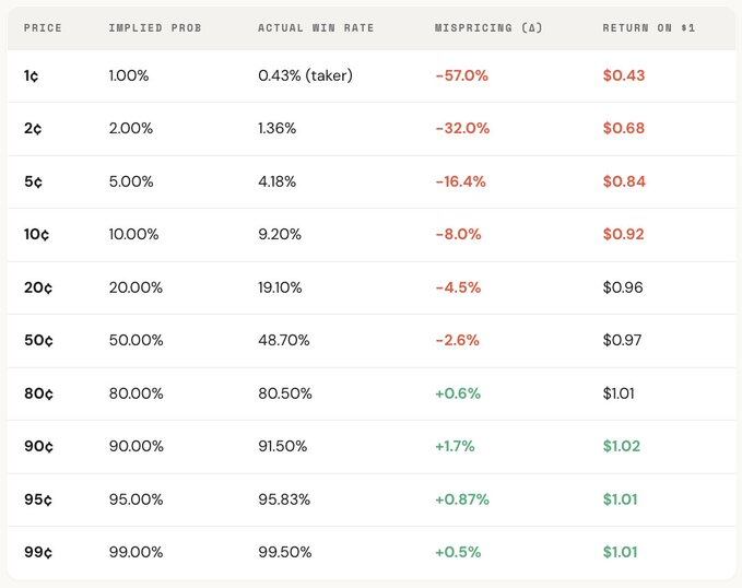

Formula 2: Single Gross Excess Return (Gross Excess Return, rᵢ)

If mispricing reflects an overall bias, then the single gross excess return reveals the actual return structure of each trade, where behavioral biases become clearly visible. When buying a $0.05 contract, two outcomes can occur: if the contract hits, the return can reach +1900% (about 20 times the return); if not, the loss is a direct 100%, with the entire $0.05 invested becoming worthless.

This is precisely why "underdog preference" is attractive; once it hits, the return is extremely high, easy to remember, amplify, and propagate. However, from an overall perspective, its actual hit rate is lower than the probabilities implied by the price, and the asymmetrical structure between “total loss” and “extremely high return” forms a negative expected value across a large number of trades, essentially equivalent to buying overpriced lottery tickets.

From an overall distribution perspective, this bias has a clear price gradient, meaning the lower the price of the contract, the worse the return. For example, as a taker, on a $0.01 contract, for every $1 invested, the average return is only about $0.43; whereas on a $0.90 contract, for every $1 invested, the average return can be about $1.02. The cheaper the price, the less favorable the actual trading conditions.

Further role breakdown reveals that this structure is almost a mirror relationship, with takers' losses in the low-price range (down to -57%) directly corresponding to makers' gains in the same range; the overall market's pricing bias is positioned between the two. In other words, every penny lost by takers is almost entirely gained by makers.

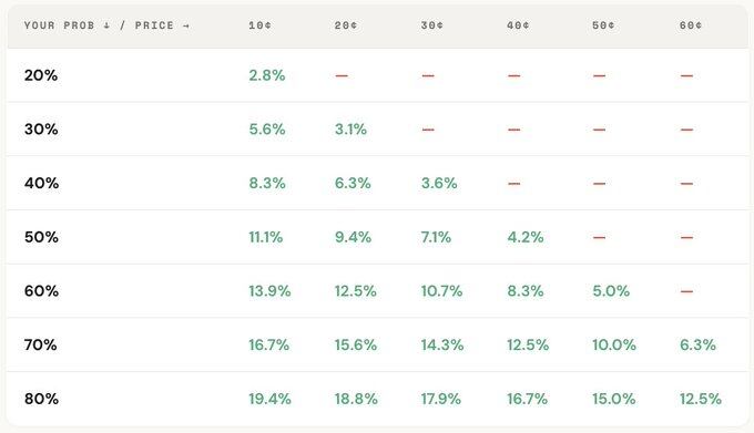
From a game theory perspective, low probability contracts are typically systematically overestimated, while high probability contracts are often underestimated. The real strategy is not to chase the underdogs, but to sell underdogs and buy high certainty.

3. Kelly Formula: How Much to Bet

When a trade with positive expected value is identified, the real question begins; how much should the trader bet? A position that is too large could wipe out weeks of earnings in a single loss; a position that is too small might grow at such a slow rate that it becomes almost meaningless. Between “all-in” and “not betting at all,” there exists a mathematically optimal betting ratio, known as the Kelly formula.

The Kelly formula was proposed by John Kelly Jr. in 1956, initially to optimize communication signal noise problems; later it has been proven to be one of the most effective position management methods in gambling, trading, and even prediction markets. Professional poker players, sports betting experts, and Wall Street quantitative funds are all using some form of Kelly strategy.

In prediction markets, since contracts have a binary structure (result is $1 or $0), and the price itself represents probability, the application of the Kelly formula is also more direct. The key lies in understanding the odds (b): if buying a YES contract at $0.30, one is actually betting $0.30 to win $0.70, which corresponds to odds of 0.70 / 0.30 ≈ 2.33; when the price is at $0.50, the odds are 1; at $0.10, the odds are 9; at $0.80, they are only 0.25. The higher the odds, the larger the recommended betting ratio by Kelly, given an advantage.

However, a key principle is not to use full Kelly. Although mathematically, full Kelly can maximize the long-term growth rate of capital, its execution can vary greatly, with drawdowns often exceeding 50%. While it may yield the highest returns over a long period, the severe volatility along the way often makes it hard for most people to stick with it. Therefore, the more common practice is to employ a fractional Kelly (like 1/2 or 1/4 Kelly). For example, under stable win rate conditions, full Kelly may yield the highest capital curve, but with extreme volatility; 1/4 Kelly will have smoother growth with controllable drawdowns; while 1/2 Kelly lies between the two.

Essentially, the Kelly formula provides a discipline, assessing first whether an advantage exists (i.e., subjective probability higher than market implied probability); and based on this, determining how much capital to invest. Only when “whether to bet” and “how much to bet” are both constrained by mathematics does trading transition from being a game to a strategy.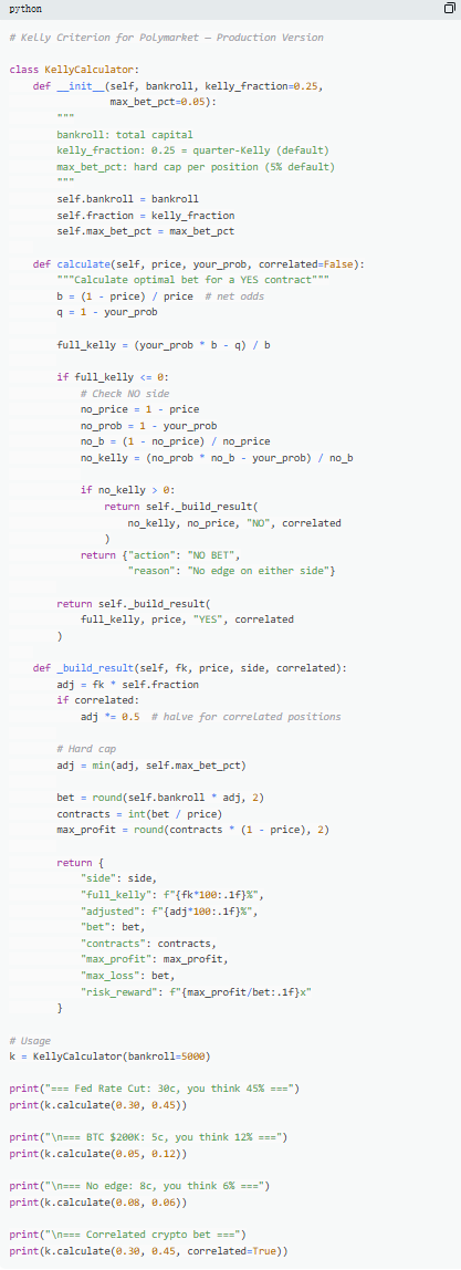

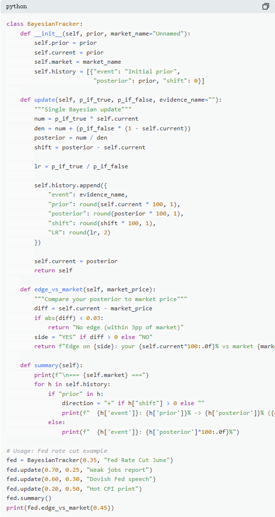
4. Bayesian Updating: Changing Perspective Like an Expert

The fluctuations in prediction markets are primarily due to the continuous influx of new information. The key is not whether the initial judgment is correct, but how to adjust perceptions when evidence changes. Most traders either ignore new information or overreact, while Bayesian updating provides a mathematical method for “how much to adjust.”

Its core logic can be simply understood as new judgment = support degree of the evidence for the original hypothesis × original judgment ÷ overall probability of that evidence. In practical applications, it is usually expanded through the total probability formula to derive a more calculable form.

For example, in a typical market, “Will the Federal Reserve lower interest rates at the June meeting?” The current market price is $0.35, corresponding to a 35% probability as the initial judgment. Then, the non-farm payroll data is released, showing an increase of only 120,000 jobs (expected 200,000), with the unemployment rate rising and wage growth slowing. In this situation, if the Federal Reserve indeed lowers rates, the probability of weak job data occurring is relatively high, estimated at 70%; if they do not lower rates, the probability of such data occurring is lower but still possible, estimated at 25%.

After substituting into Bayesian updating, the new probability is approximately 60.1%, meaning it’s a substantial revision from 35% to 60.1%, an increase of about 25 percentage points. This indicates that a key piece of information can significantly alter market judgment.

In practice, it is not necessary to calculate the complete formula each time. The more commonly used method is the “likelihood ratio.” The same piece of information (for example, LR = 3) affects differently depending on varying initial judgments: starting from 10%, it may rise to about 25%; starting from 50%, it may rise to 75%; while starting from 90%, it would only rise to about 96%. The greater the uncertainty, the larger the impact of the information.

The truly successful long-term traders in prediction markets are not necessarily the ones who make the most accurate judgments, but those who can adjust their judgments most quickly and reasonably when new evidence arises. The Bayesian method essentially provides a gauge for this “adjustment speed.”

5. Nash Equilibrium: The “Poker Formula” in Prediction Markets

In poker, bluffing is never spontaneous; it is a strategy that can be precisely calculated. There exists an optimal bluffing frequency, and once deviated from, skilled opponents can exploit it. The same logic applies to prediction markets. On Polymarket, “bluffing” corresponds to counter-trend trading—choosing to stand opposed to the majority when pricing deviates from the market; while “folding” is akin to being a passive taker, continually paying a premium for market sentiment.

On Polymarket, makers and takers form a similar adversarial relationship. Counter-trend trading (against market consensus) is similar to “bluffing,” while trend-following trading (alignment with mainstream judgments) is akin to “value betting.” From the equilibrium perspective, the market should keep marginal participants indifferent between “being a maker” and “being a taker,” corresponding to the Nash equilibrium in prediction markets.

However, this equilibrium is not fixed but dynamically adjusts with changes in participant structure. Data shows that different market categories correspond to different optimal strategies: in areas where information is more rational and pricing is more effective (like financial markets), the counter-trend space is smaller; whereas in areas with stronger emotions and greater irrationality (like entertainment and sports), market pricing biases more easily emerge, providing opportunities for counter-trend trading.

Moreover, this equilibrium has also changed significantly over time. In the early years (2021–2023), takers were actually the profitable group, with optimal strategies leaning toward active trading; after the explosive trading volume in the fourth quarter of 2024 and the large influx of professional market makers, the market structure changed, and the equilibrium strategy shifted to favor makers (about 65%–70%). This is a typical outcome of game theory; when participant structures change, optimal strategies evolve accordingly. Strategies that were effective in a “novice environment” may quickly become ineffective in front of “professional opponents,” leading to continuous iterations in the market’s “play.”

Conclusion

87% of prediction market wallets ultimately lose money not because the market is manipulated, but because these traders have never really calculated. They buy obscure contracts at prices worse than a slot machine, decide positions based on feelings, ignore changes in new information, and pay for “optimism” with every market trade.

Those 13% who can sustain profits are not simply luckier, but rather utilize these 5 formulas as a complete methodology, creating a full flow from judgment to execution, with every step based on 72 million real trade data.

This window will not remain open indefinitely. As professional market makers enter, market spreads are being rapidly compressed; the takers who once had approximately +2.0% advantage in 2022 have now turned into -1.12%.

The question is simply whether to evolve together with the market or continue buying $1 lottery tickets for a $0.43 return.

免责声明：本文章仅代表作者个人观点，不代表本平台的立场和观点。本文章仅供信息分享，不构成对任何人的任何投资建议。用户与作者之间的任何争议，与本平台无关。如网页中刊载的文章或图片涉及侵权，请提供相关的权利证明和身份证明发送邮件到support@aicoin.com，本平台相关工作人员将会进行核查。