原文作者: @BlazingKevin_ ,the Researcher at Movemaker
在加密资产市场中,交易者时常会遇到两类典型问题:一是目标交易代币的买一价与卖一价之间存在过大的差额;二是在提交大额市价订单后,资产价格出现剧烈变动,导致成交价严重偏离预期,产生高昂的滑点成本。这两类现象均由同一个根本性因素导致——市场流动性不足。而系统性地解决这一问题的核心市场参与者,即是做市商。
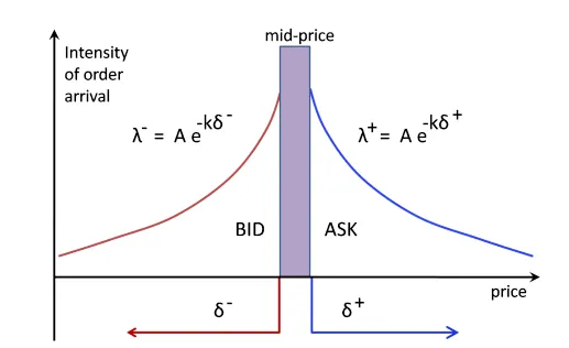
做市商的准确定义是专业的量化交易公司,其核心业务是在交易所的订单簿上,围绕资产的当前市场价格,持续地、同时性地提交密集的买入(Bid)和卖出(Ask)报价。
他们存在的根本功能,是为市场提供持续的流动性。通过双边报价行为,做市商直接缩小了买卖价差(Bid-Ask Spread),并增加了订单簿的深度。这确保了其他交易者在任何时间点的买卖意图,都能得到即时的订单匹配,从而使交易能够高效、并以一个公允的价格执行。作为此项服务的报酬,做市商的利润来源于在海量交易中获取的微小价差,以及交易所为激励流动性供给而支付的费用返还。
1011 的市场行情,使做市商的角色成为市场讨论的焦点。当价格出现极端波动时,一个关键问题浮现:做市商是被动地触发了连锁清算,还是在风险加剧时主动撤回了流动性报价?
为了分析做市商在类似情况下的行为模式,有必要首先理解其运营的基本原理。本文旨在系统性地回答以下几个核心问题:
- 做市商赖以盈利的商业模式是什么?
- 为实现其商业目标,做市商会采取何种量化策略?
- 当市场波动加剧并出现潜在风险时,做市商分别会启动哪些风险控制机制?
在厘清上述问题的基础上,我们将能够更清晰地推断出,在 1011 行情中做市商的行为逻辑与决策轨迹。
做市商的基础盈利模型
1.1 核心盈利机制:价差捕获与流动性返佣
要理解做市商在市场中的行为,首先必须知道其最根本的盈利来源。做市商通过在交易所订单簿上提供持续的双边报价(即“做市”),其利润主要由两个部分构成:捕获买卖价差与赚取交易所的流动性供给返佣。
为阐述这一机制,我们构建一个简化的合约订单簿分析模型。
来源:Movemaker
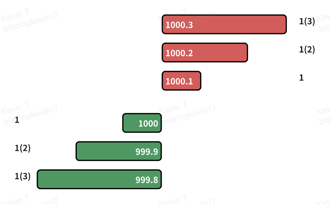
假设存在一个订单簿,其买卖盘分布如下:
- 买盘 (Bids): 密集分布于 $1000.0, $999.9, $999.8 等价位。
- 卖盘 (Asks): 密集分布于 $1000.1, $1000.2, $1000.3 等价位。
同时,我们设定以下市场参数:
- 吃单方手续费: 0.02%
- 挂单方返佣: 0.01%
- 最小价格增量: $0.1
- 当前价差 (Spread): 最优买价 ($1000.0) 与最优卖价 ($1000.1) 之间的差额为 $0.1。
1.2 交易流程与成本收益分析
现在,我们通过一个完整的交易周期来分解做市商的收益过程。
步骤一:做市商的买单被动成交 (Taker Sells)
来源:Movemaker
- 事件: 市场上一位交易者(Taker)以市价卖出一个合约,该订单与订单簿上最优的限价买单成交,即做市商在$1000.0价位挂出的买单。
- 名义成本: 从交易记录上看,做市商似乎以 $1000.0 的价格,建立了一个合约的多头头寸。
- 有效成本: 然而,由于做市商是流动性提供方(Maker),该笔交易不仅无需支付手续费,还能获得交易所0.01%的返佣。在本例中,返佣金额为 $1000.0 * 0.01% = $0.1。因此,做市商建立该多头头寸的实际资金流出(有效成本)为:$1000.0 (名义成本) - $0.1 (返佣) = $999.9。
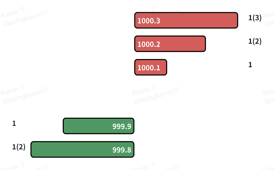
步骤二:做市商的卖单被动成交 (Taker Buys)
- 事件: 市场上一位交易者(Taker)以市价买入一个合约,该订单与订单簿上最优的限价卖单成交,即做市商在$1000.1价位挂出的卖单。此举平掉了做市商在步骤一中建立的多头头寸。
- 名义收入: 交易记录显示做市商以 $1000.1 的价格卖出。
- 有效收入: 同样,作为流动性提供方,做市商在此次卖出交易中再次获得 0.01% 的返佣,金额为 $1000.1 * 0.01% ≈ $0.1。因此,做市商平仓的实际资金流入(有效收入)为:$1000.1 (名义收入) + $0.1 (返佣) = $1000.2。
1.3 结论:真实利润的构成
通过完成这一买一卖的完整周期,做市商的单次总利润为:
总收益=有效收入−有效成本=$1000.2−$999.9=$0.3
由此可见,做市商的真实利润,并不仅仅是订单簿上可见的$0.1名义价差。其真实利润的构成是:
真实利润=名义价差+买单返利+卖单返利
$0.3=$0.1+$0.1+$0.1
这种在高频交易中,通过无数次重复上述过程来累积微小利润的模式,构成了做市商业务最基础、最核心的盈利模型。
做市商的动态策略与风险敞口
2.1 盈利模型面临的挑战:定向价格变动
前述的基础盈利模型,其有效性的前提是市场价格在一定区间内窄幅波动。然而,当市场出现明确的单边定向移动时,该模型将面临严峻挑战,并使做市商直接暴露于一种核心风险之下——逆向选择风险。
逆向选择是指,当新信息进入市场导致资产公允价值发生变化时,知情的交易者会选择性地成交做市商尚未更新的、处于“错误”价位的报价,从而使做-市商积累对其不利的头寸。
2.2 场景分析:应对价格下跌的策略抉择
为具体说明,我们延续之前的分析模型,并引入一个市场事件:资产的公允价格从 $1000 迅速下跌至 $998.0。
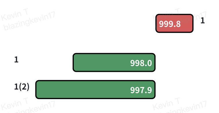
来源:Movemaker
假设做市商只持有一个在先前交易中建立的多头合约,其有效成本为 $999.9。如果做市商不采取任何行动,其在 $1000.0 附近挂出的买单将对套利者构成无风险的利润机会。因此,一旦监测到价格的定向变动,做市商必须立即做出反应,首要动作是主动撤销所有接近旧市场价格的买单。
此时,做市商面临一个策略抉择,主要有以下三种应对方案:
- 方案一:立即平仓,实现亏损做市商可以选择以市价单立即卖出持有的多头合约。假设成交在 $998.0,做市商需支付 0.02% 的吃单手续费。
- 亏损=(有效成本−退出价格) + 吃单手续费
- 亏损=($999.9−$998.0)+($998.0×0.02%)≈$1.9+$0.2=$2.1
- 此方案的目的是迅速消除风险敞口,但会立即产生确定性的亏损。
- 方案二:调整报价,寻求更优价格退出做市商可以将自己的卖一报价下调至新的市场公允价附近,例如 $998.1。如果该卖单成交,做市商将作为挂单方获得返佣。
- 亏损=(有效成本−退出价格)−挂单返利
- 亏损=($999.9−$998.1)−($998.1×0.01%)≈$1.8−$0.1=$1.7
- 此方案旨在以更小的损失退出头寸。
- 方案三:扩大价差,管理现有头寸做市商可以采取非对称的报价策略:将卖一报价调整至一个相对不具吸引力的价位(如图 $998.8),同时将新的买单挂在更低的价位(如 $998.0 和 $997.9)。 此策略的目标是通过后续的交易来管理并降低现有头寸的平均成本。
2.3 策略执行与库存风险管理
假设在“单一做市商”市场结构下,由于其拥有绝对的定价权,做市商大概率会选择方案三,以避免立即实现亏损。在该方案中,由于卖单价格 ($998.8) 远高于公允价 ($998.0),其成交概率较低。相反,更靠近公允价的买单 ($998.0) 更可能被市场上的卖方成交。
步骤一:通过增持降低平均成本
- 事件:做市商在 $998.0 挂出的买单被成交。
- 新增头寸的有效成本:$998.0 - (998.0×0.01%)≈$997.9
- 更新后的总头寸:做市商现在持有两份多头合约,其总有效成本为 999.9+$997.9=$1997.8。
- 更新后的平均成本:$1997.8 / 2 =$998.9
步骤二:基于新成本调整报价
通过上述操作,做市商成功将其多头头寸的盈亏平衡点从 $999.9 降低至 $998.9。基于这个更低的成本基础,做市商现在可以更积极地寻求卖出机会。例如,它可以将卖一报价从 $998.8 大幅下调至$998.9,在实现盈亏平衡的同时,将价差从之前的 $1.8 ($999.8 - $998.0) 显著缩小至 $0.8 ($998.8 - $998.0),以吸引买方成交。
2.4 策略的局限性与风险的暴露
然而,这种通过增持来摊薄成本的策略具有明显的局限性。如果价格继续下跌,例如从 $1000 崩跌至 $900,做市商将被迫在持续亏损的情况下不断增持,其库存风险将急剧放大。届时,继续扩大价差将导致交易完全停滞,形成恶性循环,最终不得不以巨大亏损强行平仓。
这就引出一个更深层次的问题:做市商如何定义和量化风险?不同程度的风险又与哪些核心因素相关?对这些问题的回答,是理解其在极端市场中行为的关键。
核心风险因素与动态策略制定
做市商的盈利模型,本质上是在承担特定风险以换取回报。其面临的亏损,主要源于资产价格在短期内发生大幅度的、不利于其库存头寸的偏离。因此,理解其风险管理框架,是剖析其行为逻辑的关键。
3.1 核心风险的识别与量化
做市商面临的风险,可以归结为两个相互关联的核心因子:
- 市场波动性: 这是首要的风险因子。波动性的加剧,意味着价格偏离当前均值的可能性和幅度都在增加,直接威胁到做市商的库存价值。
- 均值回归的速度: 这是第二个关键因子。在价格发生偏离后,其能否在短时间内回归至均衡水平,决定了做市商是能通过摊平成本最终盈利,还是会陷入持续的亏损。
而判断均值回归可能性的一个关键可观测指标,是交易量。在作者今年 4 月 22 号发表的文章《市场分歧加剧的回顾:反弹转变为反转,还是下跌中继的第二次派发?》提到了订单簿中的弹珠理论,不同价格的挂单根据挂单量形成了厚度不均的玻璃层,波动的市场就如同一颗弹珠。我们可以将订单簿上不同价位的限价订单,视为具有不同厚度的“流动性吸收层”。
市场的短期价格波动,则可视为一股冲击力量的弹珠。在低交易量环境下,冲击力量较弱,价格通常被限制在最密集的流动性层之间窄幅运动。而在高交易量环境下,冲击力量增强,足以击穿多层流动性。被消耗的流动性层难以瞬时补充,尤其是在单边行情中,这会导致价格向一个方向持续移动,均值回归的概率降低。因此,单位时间内的交易量,是衡量这股冲击力量强度的有效代理指标。
3.2 基于市场状态的动态策略参数化
来源:Movemaker
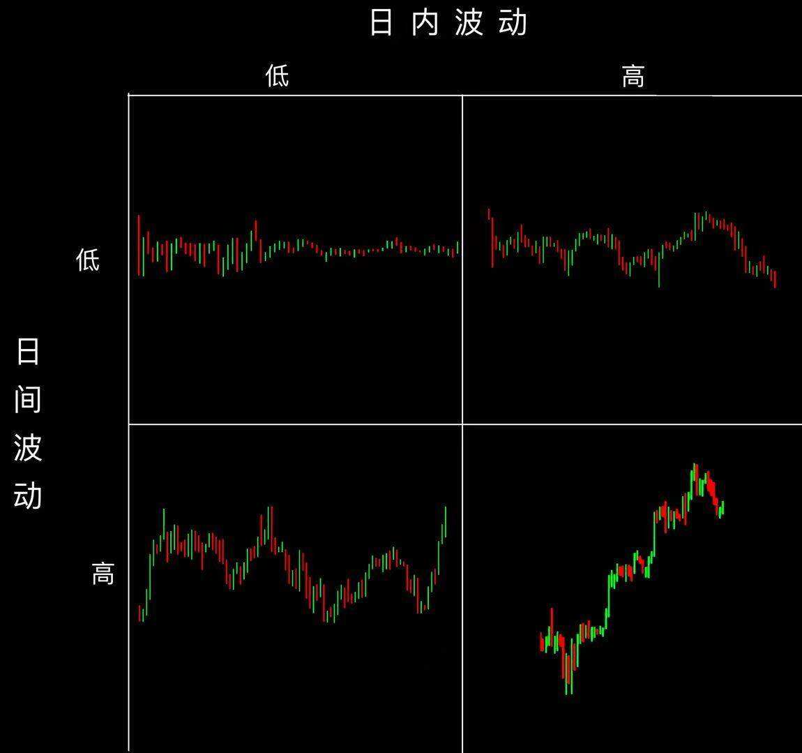
根据波动性在不同时间尺度(日内 vs. 日间)的表现,做市商会动态调整其策略参数,以适应不同的市场环境。其基础策略可以归纳为以下几种典型状态:
- 在稳定市场中,当价格的日内与日间波动均处于低位时,做市商的策略会极具进攻性。他们会采用大额订单与极窄的价差,目标是最大化交易频率和市场份额,以在低风险环境中捕获尽可能多的成交量。
- 在区间震荡市场中,当价格呈现高日内波动、但低日间波动的特征时,做市商对价格的短期均值回归抱有较高信心。因此,他们会扩大价差以获取更高的单笔利润,同时维持较大的订单规模,以便在价格波动时有足够的“弹药”进行成本摊平。
- 在趋势性市场中,当价格日内波动平稳、但日间呈现明确的单边走势时,做市商的风险敞口急剧增加。此时,策略会转向防御。他们会采用极窄的价差与小额的订单,目的是快速成交以捕获流动性,并在趋势对自身库存不利时能够迅速止损退出,避免与长期趋势对抗。
- 在极端波动市场(危机状态)中,当价格的日内与日间波动性全面加剧时,做市商的风险管理被置于首位。策略会变得极度保守,他们会显著扩大价差并使用小额订单,以极度谨慎的方式管理库存风险。在这种高风险环境下,许多竞争对手可能会退出,反而为有能力管理风险的做市商留下了潜在的机会。
3.3 策略执行的核心:公允价格发现与价差设定
无论在哪种市场状态下,做市商策略的执行都围绕两个核心任务展开:确定公允价格和设定最优价差。
- 确定公允价格这是一个不存在唯一正确答案的复杂问题。若模型有误,做市商的报价将被更知情的交易者“吃掉”,使其系统性地积累亏损头寸。常见的基础方法包括使用聚合多个交易所的指数价格,或取当前最优买卖价的中间价。最终,无论采用何种模型,做市商必须确保其报价具备市场竞争力,能够有效出清库存。长期持有大量单边头寸,是导致重大亏损的最主要原因。
- 设定最优价差设定价差的难度甚至高于发现公允价格,因为它是一个动态的、多方博弈的过程。过于激进地收窄价差,会陷入“竞争性均衡陷阱”:虽然能抢占最优报价位置,但利润空间被压缩,且一旦价格变动,极易被套利者率先成交。这要求做市商必须构建一个更智能的量化框架。
3.4 一个简化的最优价差量化框架
为阐明其内在逻辑,我们引用 Meduim 上的作者 David Holt 构建的一个简化模型,在一个高度理想化的假设下,推导最优价差。
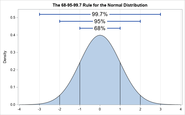
- A. 核心假设与波动性测算假设市场价格在短期内服从正态分布,以 1 秒为采样周期,考察过去 60 秒的样本数据。经计算,该样本内标记价格相对于平均中间价的标准差 (σ) 为$0.4。这意味着,在约 68% 的时间内,下一秒的价格将落在 [均值 - $0.4, 均值 + $0.4] 的区间内。
来源:Idrees
- B. 关联价差、概率与预期收益基于此,我们可以推算不同价差被成交的概率,并计算其预期收益。例如,若设定$0.8的价差(即在均值两侧各挂单 $0.4),价格需波动至少一个标准差才能触及订单,其概率约为 32%。假设每次成交能捕获半个价差($0.4),则每个时间周期的预期收益约为 $0.128 (32% × $0.4)。
来源:知乎
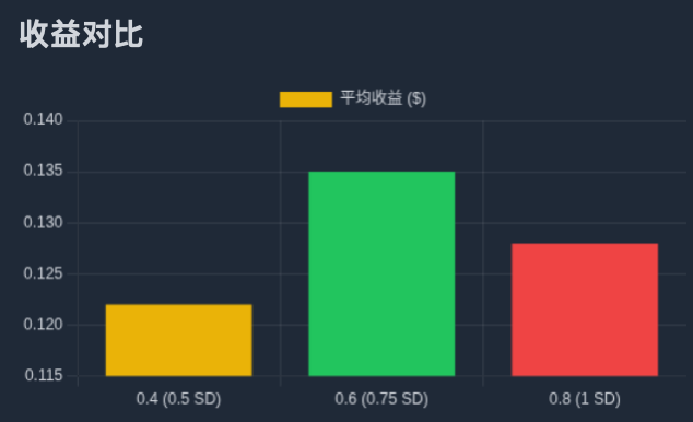
- C. 寻找最优解通过对不同价差进行迭代计算,可以发现:价差 $0.2 预期收益约 $0.08;价差 $0.4 预期收益约 $0.122;价差 $0.6 预期收益约 $0.135;价差 $0.8 预期收益约 $0.128。结论是在此模型下,最优价差为 $0.6,即在距离均价$0.3(约 0.75σ) 的位置挂单,能实现期望收益的最大化。
来源:Movemaker
3.5 从静态模型到动态现实:多时间框架风险管理
上述模型的致命缺陷是假设了均值不变。在真实市场中,价格均值会随时间漂移。因此,专业的做市商必须采用多时间框架的分层策略来管理风险。
策略的核心在于,在微观层(秒级)沿用量化模型设定最优价差,同时在中观层(分钟级)和宏观层(小时/日级)监测价格均值的漂移和波动性结构的改变。当均值发生偏移时,系统会动态地重新校准整个报价区间的中轴,并相应调整库存头寸。
这种分层模型最终导向一套动态的风险控制规则:
- 当秒级波动性增加时,自动扩大价差。
- 当中期波动性增加时,减少单笔挂单规模,但增加挂单层级,将库存分散在更宽的价格区间内。
- 当长周期趋势与库存头寸方向相反时,主动干预,如进一步削减挂单规模,甚至暂停策略,以防范系统性风险。
风险应对机制与高级策略
4.1 高频做市中的库存风险管理
前文所述的动态策略模型,属于高频做市的范畴。此类策略的核心目标是在精确管理库存风险的前提下,通过算法设定最优买卖报价,以最大化预期利润。
库存风险,被定义为做市商因持有净多头或净空头头寸,而暴露于不利价格波动下的风险。当做市商持有多头库存时,面临价格下跌的亏损风险;反之,当持有空头库存时,则面临价格上涨的亏损风险。有效管理这种风险,是做市商能否长期生存的关键。
专业的量化模型,如经典的斯托伊科夫模型 (Stoikov Model),为我们提供了一个理解其风险管理逻辑的数学框架。该模型旨在通过计算一个动态调整后的“参考价格”,来主动管理库存风险。做市商的双边报价将围绕这个新的参考价格展开,而非静态的市场中间价。其核心公式如下:
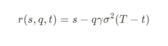
其中,各个参数的含义如下:
- r(s,q,t):动态调整后的参考价格,是做市商报价的基准中轴。
- s:当前的市场中间价。
- q:当前的库存量。若为多头则为正,空头则为负。
- γ:风险规避参数 。这是一个由做市商设定的、反映其当前风险偏好的关键变量。
- σ:资产的波动率。
- (T−t):距离交易周期结束的剩余时间。
该模型的核心思想是,当做市商的库存 (q) 偏离其目标(通常为零)时,模型会系统性地调整报价中轴,以激励市场成交能使其库存回归均衡的订单。例如,当持有多头库存 (q>0) 时,模型计算出的 r(s,q,t)将低于市场中间价 s,这意味着做市商会将其买卖报价整体下移,使得卖单更具吸引力,买单更不具吸引力,从而增加平掉多头库存的概率。
4.2 风险规避参数 (γ) 与策略的最终选择
风险规避参数 γ 是整个风险管理系统的“调节阀”。做市商会根据对市场状态的综合判断(如波动性预期、宏观事件等)来动态调整 γ 的值。在市场平稳时,γ 可能较低,策略偏向于积极赚取价差;当市场风险加剧时,γ 会被调高,使得策略极度保守,报价会显著偏离中间价以快速降低风险敞口。
在极端情况下,当市场出现最高级别的风险信号(例如,流动性枯竭、价格剧烈脱锚)时,γ 的值会变得极大。此时,模型计算出的最优策略,可能会是生成一个极度偏离市场的、几乎不可能成交的报价。在实践中,这等同于一个理性的决策——暂时性地、完全撤出流动性,以避免因无法控制的库存风险而导致灾难性亏损。
4.3 现实中的复杂策略
最后,必须强调的是,本文所讨论的模型,仅是在简化假设下对做市商核心逻辑的阐述。在真实的、高度竞争的市场环境中,顶级的做市商会采用远为复杂的、多层次的策略组合来最大化利润并管理风险。
这些高级策略包括但不限于:
- 对冲策略:做市商通常不会任由其现货库存暴露于风险之下,而是会通过在永续合约、期货或期权等衍生品市场上建立相反的头寸,来实现Delta 中性或更复杂的风险敞口管理,将其风险从价格方向风险转变为其他可控的风险因子。
- 特殊执行:在某些特定场景下,做市商的角色会超越被动的流动性提供。例如,在项目 TGE 后,他们通过TWAP (时间加权平均价格)或VWAP (成交量加权平均价格)等策略,在一定时间内出售大量代币,这构成了其重要的利润来源。
1011 复盘:风险触发与做市商的必然选择
基于前文建立的分析框架,我们现在可以对 1011 的市场剧变,进行一次的复盘。当价格呈现出剧烈的单向移动时,做市商的内部风险管理系统必然被触发。触发该系统的,可能是多重因素的叠加:某一时间框架下的平均损失超出了预设阈值;净库存头寸在极短时间内被市场上的对手方“喂满”;或是在达到最大库存限制后,无法有效出清头寸,导致系统自动执行仓位收缩程序。
5.1 数据解析:订单簿的结构性坍塌
要理解当时市场的真实情况,我们必须深入分析订单簿的微观结构。以下这张源自订单簿可视化工具的图表,为我们提供了证据:
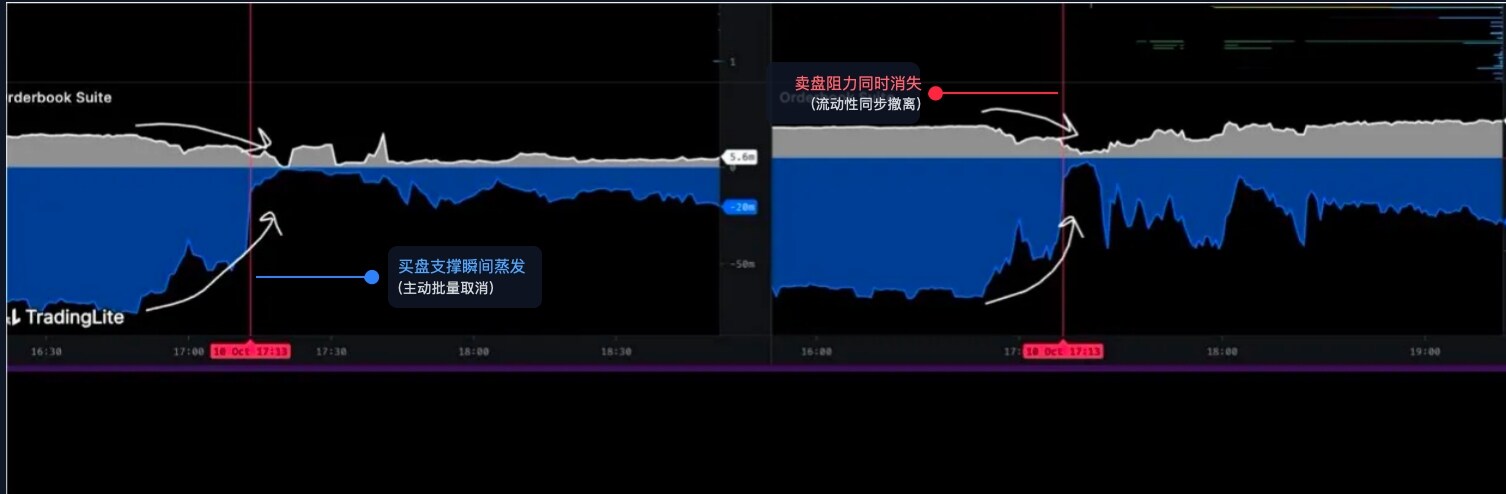
(注:为保持分析的严谨性,请将此图视为对当时市场情况的典型呈现)
这张图表直观地展示了订单簿深度随时间的变化:
- 灰色区域:代表卖盘流动性,即挂在当前价格之上、等待卖出的限价订单总和。
- 蓝色/黑色区域:代表买盘流动性 ,即挂在当前价格之下、等待买入的限价订单总和。
在图中红色竖线标记的 凌晨5:13这一精确时刻,我们能观察到两个同步发生的、异乎寻常的现象:
- 买盘支撑的瞬时蒸发:图表下方的蓝色区域出现了一个巨大的、近乎垂直的“断崖”。这种形态与买单被大量成交所消耗的情况完全不同——后者应呈现出流动性被逐级、渐次侵蚀的形态。而这种整齐划一的垂直消失,唯一合理的解释是:大量的限价买单被主动、同时、批量地取消了。
- 卖盘阻力的同步消失:图表上方的灰色区域也出现了几乎完全相同的“断崖”。大量的限价卖单在同一瞬间被主动撤离。
这一系列动作,在交易术语中被称为“流动性撤离”。它标志着市场的主要流动性提供者(主要是做市商),在极短的时间内,几乎是同步地撤回了他们的双边报价,瞬间将一个看似流动性充裕的市场,转变为一个极度脆弱的“流动性真空”。
5.2 事件的两个阶段:从主动撤离到真空形成
因此,1011 的暴跌过程,可以清晰地划分为两个逻辑递进的阶段:
第一阶段:主动的、系统性的风险规避执行
在 凌晨 5:13 之前,市场可能仍处于表面的平稳状态。但在那一刻,某个关键的风险信号被触发——这可能是一则突发的宏观消息,也可能是某个核心协议(如 USDe/LSTs)的链上风险模型发出了警报。
在接收到信号后,顶尖做市商的算法交易系统立即执行了预设的“紧急避险程序”。该程序的目标只有一个:在最短的时间内,将自身的市场风险敞口降至最低,优先于一切盈利目标。
- 为何撤销买单?这是最关键的防御性操作。做市商的系统预判到,一场规模空前的抛压即将来临。如果不立即撤走自己的买单,这些订单将成为市场的“第一道防线”,被迫承接大量即将暴跌的资产,从而造成灾难性的库存亏损。
- 为何同时撤销卖单?这同样是基于严格的风险控制原则。在波动性即将急剧放大的环境中,保留卖单同样存在风险(例如,价格可能在暴跌前出现短暂的向上“假突破”,导致卖单在不利价位被过早成交)。在机构级的风险管理框架下,最安全、最理性的选择是“清空所有报价,进入观察模式”,直到市场重新出现可预测性,再根据新的市场状况重新部署策略。
第二阶段:流动性真空的形成与价格的自由落体
在 凌晨 5:13 之后,随着订单簿“断崖”的形成,市场结构发生了根本性的质变,进入了我们所描述的“流动性真空”状态。
在主动撤离之前,要使市场价格下跌 1%,可能需要大量的卖单来消耗层层堆积的买盘。但在撤离之后,由于下方的支撑结构已不复存在,可能只需要极少数的卖单,就能造成同等甚至更为剧烈的价格冲击。
结论
1011 史诗级的市场崩盘,其直接的催化剂与放大器,正如图表所揭示的、由顶尖做市商所执行的一次大规模、同步的主动性流动性撤离。他们并非崩盘的“元凶”或始作俑者,但他们是崩盘最有效率的“执行者”和“放大器”。通过理性的、以自我保全为目的的集体行动,他们创造了一个极度脆弱的“流动性真空”,为后续的恐慌性抛售、协议脱钩压力、以及最终的中心化交易所连环清算,提供了完美的条件。
关于 Movemaker
Movemaker 是由 Aptos 基金会授权,经 Ankaa 和 BlockBooster 联合发起的首个官方社区组织,专注于推动 Aptos 华语区生态的建设与发展。作为 Aptos 在华语区的官方代表,Movemaker 致力于通过连接开发者、用户、资本及众多生态合作伙伴,打造一个多元、开放、繁荣的 Aptos 生态系统。
免责声明:
本文/博客仅供参考,代表作者的个人观点,并不代表 Movemaker 的立场。本文无意提供:(i) 投资建议或投资推荐;(ii) 购买、出售或持有数字资产的要约或招揽;或 (iii) 财务、会计、法律或税务建议。持有数字资产,包括稳定币和 NFT,风险极高,价格波动较大,甚至可能变得一文不值。您应根据自身的财务状况,仔细考虑交易或持有数字资产是否适合您。如有具体情况方面的问题,请咨询您的法律、税务或投资顾问。本文中提供的信息(包括市场数据和统计信息,若有)仅供一般参考。在编写这些数据和图表时已尽合理注意,但对其中所表达的任何事实性错误或遗漏概不负责。
免责声明:本文章仅代表作者个人观点,不代表本平台的立场和观点。本文章仅供信息分享,不构成对任何人的任何投资建议。用户与作者之间的任何争议,与本平台无关。如网页中刊载的文章或图片涉及侵权,请提供相关的权利证明和身份证明发送邮件到support@aicoin.com,本平台相关工作人员将会进行核查。


